Perlin Noise

Computing Derivatives

Very few documents on the Web and books explain the Perlin noise method intuitively; finding information on how to compute Perlin noise derivatives (especially in an analytical way) is even more challenging. Though, for those who don't know what these derivatives are and why they are helpful, let's first briefly introduce them.

A Quick Introduction to (Partial) Derivatives

Functions' derivative are often used in computer graphics. But before we give an example, let's first review what they are. If you create an image of a 2D noise and apply some regular grid on top of that image, then we may want to know how much the noise function varies along the x and y direction at each grid point (figure 1). Does this idea sound familiar already? Remember that in the previous chapter, we used the result of a 2D noise function to displace a mesh. But let's get back to what we are trying to achieve here: how do we know the rate of change of our 2D noise function along the x- or y-axis? A straightforward solution to this problem consists of taking the value of the noise at the point where you want to compute this variation (let's call this point \(Gn_x\)), the value of the noise at the point a step further to the right from \(Gn_x\) (let's call this second point \(Gn_{x+1}\)), and then subtract the second value from the first. Example: if at the grid position \(Gn_{11}\) the noise is equal to 0.1 and at that the grid position \(Gn_{12}\) the noise value is equal to 0.7, then we can assume that the noise has varied from \(Gn_{11}\) to \(Gn_{12}\) (along the x-axis) by 0.6 (figure 1). In equation form, we would write:

Technically it is best to normalize this difference so that we get consistent results regardless of the distance that separates two points on the grids (if the results are normalized, measurements made with different grid spacing can then be compared to each other). To normalize this result, we need to divide the difference by the distance between \(G_{11}\) and \(G_{12}\). So if the distance between two points on the grid is 2, for example, then we would need to write:

In mathematics, this technique is called a forward difference. Forward because we take the next computed point and subtract from it the value at the current point.

Mathematically we can formalize this concept with the following equation:

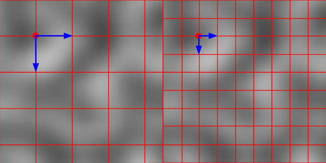
This means that we can compute the derivative of the function \(f(x)\) using the forward difference technique that we just introduced but that the value of this derivative will become more and more accurate as the distance between the two points becomes smaller (in theory \(h\) tends toward 0). When the spacing is large, you get some very crude value for the derivative at a given point \(x\), but this approximation improves as the spacing becomes small. In the case of our noise image, the grid spacing is pretty large, so you would get a much better approximation of the variation of the noise function at each point on the grid if the grid spacing was smaller (figure 2).

This concept is more easily understood with a 1D example. Figure 3 shows the profile of the one-dimensional function. Let's assume that we now want to know by how much this function varies within the proximity of P. Using the principle of forward differencing, we can take a point further down along the x-axis such as \(x_1\), compute the value of the function at that point and then subtract \(f(x_1)\) to \(f(x)\). Note that when we trace a line from \(f(x)\) to\(f(x_1)\), that line is tangent to the function at \(x\). That's because the derivative of a one-dimensional function gives the slope of the line tangent to the function where the function's derivative is being computed. So now that we know how to interpret the derivative of a function geometrically, you can easily see that if we take a point further away than \(x_1\), such as, for example, \(x_2\), then the line between \(x\) and \(x_2\) is not "as tangent" to \(x\) than is the line \(x\)-\(x_1\). In conclusion, if you use the forward difference to compute the derivative of a function, then the smaller the distance between \(x\) and \(x+h\), the better.

What have we learned so far?

• We learned that the derivative \(f'(x)\) of a one-dimensional function \(f(x)\) can be interpreted as the slope of the line tangent to the function \(f(x)\) at \(x\)

  Besides the slope, the derivative \(f'(x)\) can also be considered as the instantaneous rate of change of the function \(f(x)\) at \(x\).

• We also learned that we could use a technique called forward difference (the general method is called finite difference) to compute an "approximation" of that slope, but also that this approximation gets better as \(h\) in the forward difference equation gets smaller.

There is something significant to understand to make sense of how we will use derivatives (actually partial derivatives) later in this chapter. So far, we have explained that the derivative of a function can be interpreted as the slope of the function \(f(x)\) at any value of \(x\). The way we trace the tangent at \(x\) (where we computed the derivative of the function \(f(x)\)) is by simply drawing the line \(y = mx\) at the point on the function where we computed the derivative of the function. The value \(m\) here is, of course, the slope of the function derivative we calculated. Why is this important? It's essential because note that when \(x=1\), then \(y=m\). Using this observation, we can say that the 2D vector tangent to the curve at the point where we evaluated the derivative is equal to Vec2f(1, m). Do you agree? Of course, you then need to normalize this vector but note how this vector is tangent to the point where we evaluated the function's derivative (and that's what we want you to remember). You must understand this idea (which is illustrated in Figure 4).

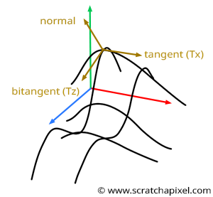
You can see the 3D Perlin noise function as two 2D functions perpendicular to each other at the point where the derivative is computed. So you will have a 1D function to compute the derivative of the 2D function in the xy plane if you wish and another 1D function to calculate the derivative of the 2D noise function in the yz plane, as shown in Figure 5. Now, if we apply the technique, we just learned to compute the tangent at each of these functions, noting that the two obtained tangents are perpendicular to each other. But more interestingly, by now taking the cross product of these two vectors, you get a vector that is perpendicular to the plane tangent to the point where the 2D noise function derivative was computed initially (as shown again in figure 5). This vector is normal of our function at P. Hopefully, by now, you will get it. These derivatives will help compute the normals of our mesh displaced by a 3D or 2D noise function.

This is simple and elegant. Now one remark and one question.

Remark: note that we don't compute the derivative of the noise function here. We cheat by computing a derivative of the function along the x-axis and then another derivative along the z-axis. What's interesting when we do that is that only one of the quantities varies. For example, when computing the derivative of the 3D noise function along the x-axis, then, of course, the value we get doesn't change because of a variation of the noise along the z-axis (since we evaluate the noise function in the plane xy - aka there's no variation in z). In mathematics, when you have a function with several variables but that you compute its derivative with respect to one of its variables only, with the others held constant. We say that we compute the function's partial derivatives. Let's take an example if you have the function:

Then if you wish to compute the derivative of the function while holding \(y\) constant, you get:

which you can read as the function \(f(x,y)\) partial derivative with respect to \(x\). In other words, we ignore all the terms in which \(x\) doesn't show up, such as \(y^2\) in our example (including any constant term), then compute the derivative of \(x\) for each term in which \(x\) shows up. For example, if in one of the terms we have a \(x^2y\), then we replace it in the partial derivative by \(2xy\). If we have \(xy\), we replace the term in the partial derivative with \(y\). Simple?

Question: how do we compute these partial derivatives, then?

One method consists of using the forward difference technique (which is why we learned about it at the beginning of this chapter). If we take the example of our displaced meshed, then we can compute the derivate along the x-axis at the vertex \(V_{x,z}\) by subtracting the derivate from the noise value at the vertex \(V_{x+1,z}\) at the vertex \(V_{x,z}\) (figure 6). In other words, we can write:

Where \(\partial Nx\) is the partial derivative of the noise function along the x-axis. This is a real value, not a vector, at this point. We can similarly compute the partial derivative of the noise function along the z-axis:

How do we transform this real value (in other words, a float) into a vector (the vector tangent to the noise function at the point where the derivative is computed along the x- and z-axis)? Well, this is simple. Remember that when we compute the partial derivative along the x-axis, we work in the xy plane. Thus the z-coordinate of the vector tangent to the noise function along the x-axis is necessarily 0:

To compute the other two coordinates, you need to look at figure 4 again, where we explained that to compute the tangent to the function in a plane, you need to set the x coordinate to 1 and the y coordinate of the vector to function partial derivative value (if you want to compute the tangent of the vector in the yz plane then you need to set the z-coordinate of the tangent to 1, the y-coordinate of the vector to the function partial derivative with respect to z, and then the x-coordinate of the tangent vector to 0). Finally, we have:

Finally, to compute the normal of the vertex, all you need to do now is to compute the cross product of these two vectors (the result of the cross product will be correct even if the two input vectors are not normalized: the resulting vector will be perpendicular to the two input vectors, though it might not be normalized itself):

This technique works great but:

• First, what happens when we want to compute the derivatives for the vertices at the grid's edges? Well, you can't.

• We also explained (figure 3) that the smaller the space between two samples when we compute the derivative using a forward difference, the more accurate the result. In other words, the larger the space between the vertices, the less accurate the computation of the partial derivatives. Later in this chapter, we will show the difference between the partial derivative computed with a forward difference and the analytical solution we will now study.

Analytical Partial Derivatives of the Perlin Noise Function

So there is a better way of computing these partial derivatives. This technique only relies on maths and provides an "accurate" solution (in the mathematical sense of the term). A quick reminder: the partial derivative of the following equation:

with respect to x is:

Let's re-write the Noise function. Let's first replace all the dot products with letters (as shown below):

a = dot(c000, p000)
b = dot(c100, p100)
c = dot(c010, p010)
d = dot(c110, p110) 
e = dot(c001, p001)
f = dot(c101, p101) 
g = dot(c011, p011)
h = dot(c111, p111)

For the sake of the exercise, let's recall that the parameters \(u\), \(v\), and \(w\) are computed as follows (we use the smoothstep function):

u = tx * tx * (3 - 2 * tx)
v = ty * ty * (3 - 2 * ty)
w = tz * tz * (3 - 2 * tz)

Let's now write the different interpolations of the Perlin noise function into one single line (see the first chapter):

lerp(
   lerp(
       lerp(a, b, u),
       lerp(c, d, u),
       v)
   lerp(
       lerp(e, f, u),
       lerp(g, h, u),
       v),
   w)

Let's now replace the call to the lerp(a, b, t) function with its actual code (a(1-t)+bt) and develop:

((a(1 - u) + bu)(1 - v) + (c(1 - u) + du)v)(1 - w) +
((e(1 - u) + fu)(1 - v) + (g(1 - u) + hu)v)w

((a - au + bu)(1 - v) + (c - cu + du)v)(1 - w) +
((e - eu + fu)(1 - v) + (g - gu + hu)v)w

(a - au + bu - av + auv - buv + cv - cuv + duv)(1 - w) +
(e - eu + fu - ev + euv - fuv + gv - guv + huv)w

a - au + bu - av + auv - buv + cv - cuv + duv -
aw + auw - buw + avw - auvw + buvw - cvw + cuvw - duvw +
ew - euw + fuw - evw + euvw - fuvw + gvw - guvw + huvw

And then, finally, regroup the terms as follows:

a + u(b - a) + v(c - a) + w(e - a) +
uv(a + d - b - c) + uw(a + f - b - e) + vw(a + g - c - e) +
uvw(b + c + e + h - a - d - f - g)

As you can see (and as expected), this is a function of three variables: \(u\), \(v\), and \(w\). Suppose we apply the technique we learned to compute the partial derivative of a function with respect to one of its variables. In that case, we need to remove all the terms that do not contain the variable in question and then replace the variable with its derivative in the remaining terms. For example, if we wish to compute the noise function partial derivative with respect to \(u\), we get:

u'(b - a) +
u'v(a + d - b - c) + u'w(a + f - b - e) +
u'vw(b + c + e + h - a - d - f - g)

u'((b - a) + v(a + d - b - c) + w(a + f - b - e) + vw(b + c + e + h - a - d - f - g))

Similarly, the partial derivatives with respect to \(v\) and \(w\) are:

// partial derivative with respect to v
v'(c - a) +
uv'(a + d - b - c) + v'w(a + g - c - e) +
uv'w(b + c + e + h - a - d - f - g)

v'((c - a) + u(a + d - b - c) + w(a + g - c - e) + uw(b + c + e + h - a - d - f - g))

// partial derivative with respect to w
w'(e - a) +
uw'(a + f - b - e) + vw'(a + g - c - e) +
uvw'(b + c + e + h - a - d - f - g)

w'((e - a)  + u(a + f - b - e) + v(a + g - c - e) + uv(b + c + e + h - a - d - f - g))

The remaining question is what is the derivative of \(u'\), \(v'\) and \(w'\)? Well simple \(u\), \(v\) and \(w\) are computed as follows:

Thus the derivatives of these functions are:

Et voila! All you need to do now is compute these derivatives and then construct the vectors tangent to the point where the function is evaluated using the abovementioned technique. Here is a modified version of our eval function that evaluates the 3D noise function and its partial derivatives at a given location:

float eval(const Vec3f &p, Vec3f& derivs) const 
{ 
    int xi = static_cast<int>(std::floor(p.x)) & tableSizeMask; 
    int yi = static_cast<int>(std::floor(p.y)) & tableSizeMask; 
    int zi = static_cast<int>(std::floor(p.z)) & tableSizeMask; 
 
    float tx = p.x - xi; 
    float ty = p.y - yi; 
    float tz = p.z - zi; 
 
    float u = smoothstep(tx); 
    float v = smoothstep(ty); 
    float w = smoothstep(tz); 
 
    float du = smoothstepDeriv(tx); 
    float dv = smoothstepDeriv(ty); 
    float dw = smoothstepDeriv(tz); 
 
    // gradients at the corner of the cell
    const Vec3f &c000 = gradients[hash(xi, yi, zi)]; 
    const Vec3f &c100 = gradients[hash(xi + 1, yi, zi)]; 
    const Vec3f &c010 = gradients[hash(xi, yi + 1, zi)]; 
    const Vec3f &c110 = gradients[hash(xi + 1, yi + 1, zi)]; 
 
    const Vec3f &c001 = gradients[hash(xi, yi, zi + 1)]; 
    const Vec3f &c101 = gradients[hash(xi + 1, yi, zi + 1)]; 
    const Vec3f &c011 = gradients[hash(xi, yi + 1, zi + 1)]; 
    const Vec3f &c111 = gradients[hash(xi + 1, yi + 1, zi + 1)]; 
 
    // generate vectors going from the grid points to p
    float x0 = tx, x1 = tx - 1; 
    float y0 = ty, y1 = ty - 1; 
    float z0 = tz, z1 = tz - 1; 
 
    Vec3f p000 = Vec3f(x0, y0, z0); 
    Vec3f p100 = Vec3f(x1, y0, z0); 
    Vec3f p010 = Vec3f(x0, y1, z0); 
    Vec3f p110 = Vec3f(x1, y1, z0); 
 
    Vec3f p001 = Vec3f(x0, y0, z1); 
    Vec3f p101 = Vec3f(x1, y0, z1); 
    Vec3f p011 = Vec3f(x0, y1, z1); 
    Vec3f p111 = Vec3f(x1, y1, z1); 
 
    float a = dot(c000, p000); 
    float b = dot(c100, p100); 
    float c = dot(c010, p010); 
    float d = dot(c110, p110); 
    float e = dot(c001, p001); 
    float f = dot(c101, p101); 
    float g = dot(c011, p011); 
    float h = dot(c111, p111); 
 
    float k0 = (b - a); 
    float k1 = (c - a); 
    float k2 = (e - a); 
    float k3 = (a + d - b - c); 
    float k4 = (a + f - b - e); 
    float k5 = (a + g - c - e); 
    float k6 = (b + c + e + h - a - d - f - g); 
 
    derivs.x = du *(k0 + v * k3 + w * k4 + v * w * k6); 
    derivs.y = dv *(k1 + u * k3 + w * k5 + u * w * k6); 
    derivs.z = dw *(k2 + u * k4 + v * k5 + u * v * k6); 
 
    return a + u * k0 + v * k1 + w * k2 + u * v * k3 + u * w * k4 + v * w * k5 + u * v * w * k6; 
}

Analytical Solution vs. Forward Difference

We can now compete for two versions of the displaced mesh, one using the geometric solution to compute the vertex normals of the mesh and one using the analytic solution. To code to compute either one of these solutions is as follows:

int main(int argc, char **argv) 
{ 
    PerlinNoise noise; 
 
    PolyMesh *poly = createPolyMesh(3, 3, 30, 30); 
 
    // displace and compute analytical normal using noise function partial derivatives
    Vec3f derivs; 
    for (uint32_t i = 0; i < poly->numVertices; ++i) { 
        Vec3f p((poly->vertices[i].x + 0.5), 0, (poly->vertices[i].z + 0.5)); 
        // displace current vertex
        poly->vertices[i].y = noise.eval(p, derivs); 
#if ANALYTICAL_NORMALS 
        Vec3f tangent(1, derivs.x, 0);  //tangent 
        Vec3f bitangent(0, derivs.z, 1);  //bitangent 
        // equivalent to bitangent.cross(tangent)
        poly->normals[i] = Vec3f(-derivs.x, 1, -derivs.z); 
        poly->normals[i].normalize(); 
#endif 
    } 
 
#if !ANALYTICAL_NORMALS 
    // compute face normal if you want
    for (uint32_t k = 0, off = 0; k < poly->numFaces; ++k) { 
        uint32_t nverts = poly->faceArray[k]; 
        const Vec3f &va = poly->vertices[poly->verticesArray[off]]; 
        const Vec3f &vb = poly->vertices[poly->verticesArray[off + 1]]; 
        const Vec3f &vc = poly->vertices[poly->verticesArray[off + nverts - 1]]; 
 
        Vec3f tangent = vb - va; 
        Vec3f bitangent = vc - va; 
 
        poly->normals[poly->verticesArray[off]] = bitangent.cross(tangent); 
        poly->normals[poly->verticesArray[off]].normalize(); 
 
        off += nverts; 
    } 
#endif 
 
    poly->exportToObj(); 
    delete poly; 
 
    return 0; 
} 

Here is an image of these two meshes with their associate vertex normals (displayed on the right):

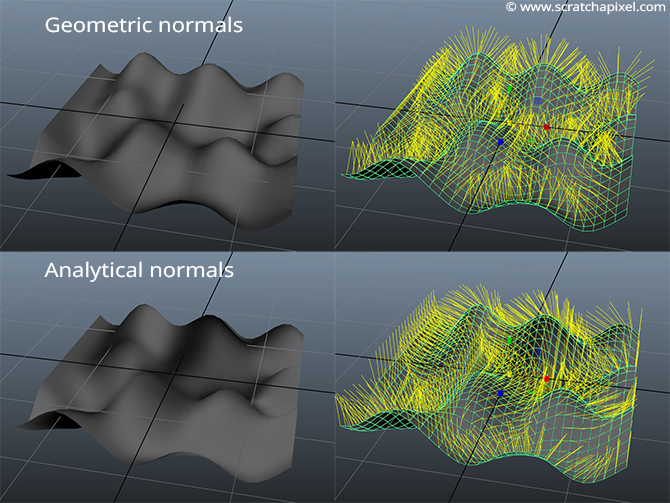
Note that the vertex normals are not defined at the edge of the mesh whose normals were computed using the forward difference method (geometric solution). Note also the directions of the vertex normals are significantly different between the two meshes (even though their shape is the same). This causes the shading of the two meshes to be noticeably different (remember that normals are used in shading).

poly->normals[i] = bitangent.cross(tangent);

poly->normals[i] = Vec3f(-derivs.x, 1, -derivs.z);