A Minimal Ray-Tracer

Parametric and Implicit Surfaces

Reading time: 11 mins.

Introduction

In the previous lesson, we learned how to generate primary rays. However, we have not yet produced an image because we have not learned how to calculate the intersection of these primary rays with any geometry. In this lesson, we will explore computing the ray-geometry intersection for simple shapes, such as spheres. Spheres are relatively straightforward to ray-trace, making them a common choice for those learning to program a ray tracer. Thus, this lesson will cover a somewhat eclectic mix of topics:

In this chapter, we delve into parametric and implicit surfaces. These surfaces, or shapes, are unique because they can be defined mathematically. This foundational knowledge will support the techniques we will explore in the next chapter to calculate their intersection with rays.
Chapter 2 introduces several methods for calculating the intersection of a ray with a sphere.
Chapter 3 combines the insights from the previous lesson on generating primary rays with the methods learned in Chapter 2 of this lesson to determine whether primary rays intersect any of the spheres comprising the scene. The program we develop in this lesson will serve as the basis for a minimal but functional ray tracer. We will first explore the trace() function, where we test each sphere against the primary ray and return the intersection distance and a pointer to the closest intersected sphere (if any intersection occurs). Then, in the castRay() function, we will learn to utilize the normal and texture coordinates at the intersection point to implement basic shading.
Chapters 4 and 5 introduce various techniques for calculating the intersection of a ray with other simple shapes, such as planes, disks, and axis-aligned boxes.
As is customary, the final chapter of this lesson provides the complete source code for all programs developed in this lesson, including instructions on how to compile them.

Ray-Geometry Intersection

In the previous lesson, we learned how to generate primary rays. Now, we must explore the ray-geometry intersection to enable image production. The goal is to apply mathematics to determine if a ray intersects an object. As previously discussed, geometry or 3D objects can be represented in several ways in computer graphics. For instance, we have mentioned polygon meshes (composed of faces), NURBS surfaces, subdivision surfaces, etc. However, apart from triangular meshes, which are a subset of polygon meshes, we have yet to study NURBS and subdivision surfaces.

These types of geometry are beneficial in computer graphics for depicting the shapes of complex objects. Simple shapes, such as spheres, planes, disks, or boxes, can be rendered more directly using simpler methods. These shapes can be mathematically described by equations, which we can then use to analytically calculate whether a ray intersects them. This lesson will cover these mathematical definitions, focusing on two main approaches: parametrically and implicitly.

Parametric Surfaces

**Figure 1:** Parametric definition of a ray.

Recall from the previous lesson that rays can also be defined using the following parametric equation:

$$P = O + tD$$

Where $P$ is a point on the ray's half-line, $O$ is the ray's origin, and $D$ is the ray's direction. The term $t$ is known as a parameter. By varying the value of $t$, we can describe numerous points on the ray's half-line, and the collection of these points forms the half-line itself. In essence, it describes the generation of an ordered sequence of points along the ray. Spheres can also be defined using a parametric form. Below is the parametric equation of a sphere:

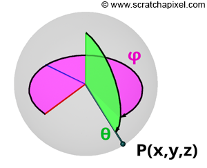
$$ \begin{array}{l} P.x = \cos(\theta)\sin(\phi),\\ P.y = \sin(\theta),\\ P.z = \cos(\theta)\sin(\phi).\\ \end{array} $$

The equations for calculating Cartesian coordinates from spherical coordinates may vary from source to source. This variance depends on the convention used for naming the coordinate system axes and whether $\theta$ denotes the polar or azimuthal angle. In the example above, $y$ is the up-axis, $x$ points to the right, and $z$ is in a plane perpendicular to $y$. Here, $\theta$ defines the polar angle, as illustrated in Figure 2.

**Figure 2:** Parametric definition of a sphere.

Or, alternatively:

$$ \begin{array}{l} \vec r(\theta,\phi) = (\cos\theta \sin\phi, \sin\theta, \cos\theta \sin\phi), \\ 0 \leq \theta < 2\pi, 0 \leq \phi \leq \pi. \end{array} $$

Where $\theta$ and $\phi$ represent a point's latitude and longitude coordinates on a sphere, defined in radians. The angle $\theta$ (the Greek letter theta) is confined to the range $[0, \pi]$, and the angle $\phi$ (the Greek letter phi) to the range $[0, 2\pi]$. We have previously introduced these equations in the lesson on Geometry. The coordinates $\theta, \phi$ of a point on a sphere, also known as spherical coordinates, are essential for understanding that a sphere can be described using a set of three equations. In these parametric equations, $\theta$ and $\phi$ serve as the parameters. 3D objects that can be defined using such equations are termed parametric surfaces.

In computer graphics (CG), this representation is advantageous because the two parameters, $\theta$ and $\phi$, often denoted as $u$ and $v$ or $s$ and $t$ in generic cases, can be used as the texture coordinates of a point on a 3D surface of the object. For instance, in the case of a sphere, we can conveniently remap the two parameters $\theta$ and $\phi$ to the range [0, 1] and utilize these coordinates to perform a lookup in a texture or generate a pattern using a procedural approach. An example of this technique will be provided in this lesson (chapter 3). In essence, the process can be viewed as mapping from 2D space to 3D space, using the 2D coordinates for texturing, as our $s$ and $t$ coordinates.

In summary, it is important to remember that parametric surfaces require one parameter to describe a curve and two parameters to describe a 3D surface.

Implicit Surfaces

**Figure 3:** Implicit form of a circle with radius $r$.

Implicit surfaces share similarities with parametric surfaces. As a starting point, consider the example of a circle defined in its implicit form by the equation:

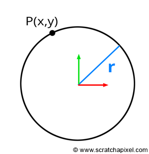
$$x^2 + y^2 = r^2.$$

Here, $x$ and $y$ represent the coordinates of a point in 2D space, and $r$ denotes the circle's radius (Figure 1). This equation holds true for any point lying on a circle with radius $r$. In other words, if you take the coordinates of any point on the circle, square them, and sum them, the result equals the square of the circle's radius. By default, this example assumes the circle is centered at the origin. However, you can generalize this equation for circles centered at arbitrary positions:

$$(x - O_x)^2 + (y - O_y)^2 = r^2.$$

Here, $O$ represents the circle's center position. This modification simply translates the circle's center to the origin. The above is the implicit equation for a circle. Extending this concept to 3D, the implicit equation for a sphere is:

$$x^2 + y^2 + z^2 = r^2.$$

The principle remains the same: the equation is true for all points lying on a sphere with radius $r$.

**Figure 4:** Using a sphere as a bounding volume to determine if a ray might intersect the enclosed geometry. If the ray does not intersect the sphere, then it cannot intersect the object within.

This lesson will explore how these equations can be utilized to test for intersections between a ray and an implicit surface.

Various shapes, such as planes, spheres, cones, and tori, can be defined with such equations. While these shapes may seem less useful for depicting complex objects—a point acknowledged at the start of this lesson—they have valuable applications. For instance, spheres can encapsulate an object's overall volume as a bounding volume (Figure 4). Testing a ray's intersection with a complex object can be computationally demanding. By first checking for an intersection with the bounding sphere, we can bypass the need to test against the object directly if the ray misses the sphere, thus saving computational time. This approach is beneficial if the time required to test a ray-sphere intersection is less than that for a ray-object intersection. Given that the cost of intersecting a ray with an implicit surface often undercuts that of a ray-triangle intersection, employing this simple ray-geometry acceleration technique can significantly reduce computation time for scenes containing many complex objects. Consequently, understanding implicit surfaces and their utility in calculating ray-geometry intersections remains valuable, despite the apparent simplicity of their forms.

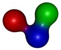
Implicit surfaces and Blobies: A fascinating category of implicit surfaces includes what are commonly referred to in CG literature as blobies or metaballs. Blobies can be envisioned as small spheres that affect each other's shape. Bringing two blobies close together causes their surfaces to blend in the middle, forming a larger, unified blob. This modeling technique, particularly popular in the 1980s and 1990s, excels at creating organic shapes. However, blobies typically require conversion into a polygon mesh before they can be easily ray-traced. Additional insights into blobies can be found in the modeling section.

Why Are These Surfaces Useful in Ray-Tracing?

The focus of this lesson is to explore how the property of being definable by an equation facilitates the calculation of ray-geometry intersection tests. While implicit surfaces are somewhat less versatile than parametric surfaces in performing these intersection tests, they prove invaluable for computing the texture coordinates of a point on the surface of an implicit object, as we'll explain in the next chapter. Therefore, understanding both representations is beneficial and necessary. Furthermore, these surfaces offer several advantages previously mentioned:

The solution to a ray-implicit surface intersection is often simpler to compute than with other types of geometry.
The calculation of a ray's intersection with an implicit surface is typically faster than with other geometry types.
Although the shapes are too simplistic to represent complex objects directly, they can serve as bounding volumes, which help accelerate ray-geometry intersection testing.
Ray-implicit surface intersection tests exemplify the practical application of mathematical concepts, such as solving the roots of a quadratic equation.

This lesson will cover the intersection tests between rays and spheres, planes, disks (an extension of the ray-plane case), and boxes. Spheres are part of a group of surfaces known as quadrics. Any quadric surface (including cones, tori, etc.) can be subjected to a ray intersection test using a method similar to the one described for spheres.

Integrate and Differentiate: Derivatives, Tangents, and Normal Vectors

Another benefit of parametric or implicit surfaces is that their defining equations can be used to compute additional useful values, such as derivatives, tangents, bi-tangents, and normals at any point on the surface. Normals play a crucial role in shading, while derivatives are important for operations like texture filtering. Tangents and bi-tangents can be employed to establish a local coordinate system at any surface point, aiding in shading. The mathematics involved in calculating these values can be substantially more complex than those used to compute ray and implicit surface intersections. Thus, they will not be covered in this lesson. Those interested in this subject may seek information on differential geometry online. A separate lesson will be dedicated exclusively to this topic. Although we will discuss normals in upcoming lessons, calculating them for shapes like spheres and triangles is simpler and does not require advanced differential geometry techniques.

About Ray-Tracing Spheres and Writing a Production-Quality Ray-Tracer

The technique we will study in this lesson for determining the intersection of a ray with a sphere differs from the method we will examine in the next lesson for the ray-triangle intersection. As discussed in a previous lesson, supporting multiple geometry types in a renderer is generally avoided for several reasons. Firstly, it necessitates additional coding. More critically, however, each program feature (such as motion blur, displacement, texture mapping, and acceleration structures) must be compatible with every supported geometry type, imposing extra constraints on the programmer. Hence, it is usually preferable to support a single geometry type (with triangles being the most common choice) and convert other geometry types to this standard form. Most production renderers can render simple shapes like spheres and tori by internally converting these shapes into polygon meshes (typically utilizing their parametric representations) rather than implementing specific ray-geometry intersection routines for each shape. In practice, rendering spheres directly is rare in production environments. Unlike the method discussed in this lesson, the traditional or native approach to ray-tracing these shapes does not require converting them into polygon meshes, offering the advantage of faster rendering compared to ray-tracing a sphere composed of hundreds or thousands of triangles. Learning to ray-trace spheres or quadric surfaces provides a valuable exercise, although, in practical terms, the approach differs from that employed in production-quality renderers.