Geometry

Spherical Coordinates and Trigonometric Functions

Reading time: 13 mins.

In addition to understanding points, vectors, normals, and matrices, mastering the concept of expressing vectors in spherical coordinates proves immensely valuable in image rendering (and CG in general). While it's possible to render images without this knowledge, incorporating spherical coordinates often simplifies complex shading challenges. This chapter also serves as a prime opportunity to revisit trigonometric functions, crucial for navigating geometric problems in computer graphics.

Trigonometric Functions

Trigonometry and the Pythagorean theorem are foundational to creating computer-generated imagery, as rendering is fundamentally a geometric endeavor. Starting with the sine and cosine functions, we'll explore how to determine angles from 2D coordinates. These functions are typically defined with respect to the unit circle, a circle with a radius of one. For a point $P$ on this circle, the $x$ -coordinate is found using the cosine of the angle ( $θ$ ) formed by the $x$ -axis and a line from the origin to $P$ . Similarly, the $y$ -coordinate is obtained using the sine of $θ$ . It's important to note that $θ$ is measured in radians, and although angles may be easier to conceptualize in degrees, a conversion to radians is necessary for computation in C++:

θ_{r a d i a n s} = \frac{π}{180} θ_{d e g r e e s}

Where a full circle's rotation (360 degrees) equals $2 π$ radians.

Trigonometric functions also stem from the relationships between the sides of a right triangle. The tangent of an angle, for example, is the ratio of the opposite side to the adjacent side of the triangle. The arctangent function, or the inverse of tangent, is particularly useful in graphics programming. While the atan function calculates the arctangent, it doesn't account for the quadrant of the angle, potentially leading to inaccuracies. The atan2 function, however, considers the signs of both $x$ and $y$ coordinates, accurately determining the angle $θ$ . For a point with coordinates (0.707, 0.707), $θ$ is $π / 4$ , whereas for (-0.707, -0.707), $θ$ should logically be $3 π / 4$ , a distinction properly handled by atan2.

Summarizing the trigonometric functions discussed:

\sin (θ) = \frac{opposite side}{hypothenuse}, \cos (θ) = \frac{adjacent side}{hypothenuse}, \tan (θ) = \frac{opposite side}{adjacent side}

And their inverse functions used to find angles given a point $P$ :

θ = acos (P_{x}), θ = asin (P_{y}), θ = atan2 (P_{y}, P_{x})

The atan2 function uniquely returns angles in the range $[- π, π]$ , with positive values for counter-clockwise angles and negative for clockwise, providing a comprehensive understanding of angle orientation.

Finally, the Pythagorean theorem, essential for various calculations such as ray-sphere intersections, states:

{hypothenuse}^{2} = {adjacent}^{2} + {opposite}^{2}

This principle asserts that the square of the length of the hypotenuse of a right triangle is equal to the sum of the squares of the triangle's other two sides.

Representing Vectors with Spherical Coordinates

**Figure 3:** a vector can also be represented by two angles: the vertical angle (in red) $θ$ and the horizontal angle (in green) $ϕ$ .

**Figure 4:** in the top figure, we are looking perpendicularly to the plane defined by the vector and the up-axis. In the bottom figure, we are looking at the vector from the top. The angle $θ$ (top figure) can vary from 0 to $π$ and the angle $ϕ$ (bottom figure) can vary from 0 to $2 π$ .

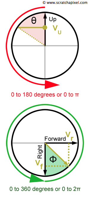
Vectors, commonly represented in Cartesian coordinates by three values corresponding to each axis, can alternatively be described using spherical coordinates, which utilize just two angles. These are the vertical angle ( $θ$ ), shown in red, and the horizontal angle ( $ϕ$ ), depicted in green, as illustrated in the accompanying figures. The vertical angle, $θ$ , measures the vector's deviation from the vertical axis, while the horizontal angle, $ϕ$ , gauges the angle between the vector's projection onto the horizontal plane and a predefined right vector of the Cartesian system.

Consistently within the computer graphics (CG) community, $θ$ denotes the vertical angle, and $ϕ$ represents the horizontal angle, a convention that aids in maintaining clarity across different texts and applications. These angles are measured in radians, with $θ$ spanning from 0 to $π$ and $ϕ$ from 0 to $2 π$ , encompassing a full circle around the axis. This method of vector representation, referred to as spherical coordinates, offers a compact way to encode direction, reducing the information needed from three values to two, provided the vector's length is not of concern.

Spherical coordinates not only simplify the representation but also play a crucial role in shading techniques, where understanding the direction relative to light sources and surfaces is key. The transition from Cartesian to spherical coordinates involves recognizing the vector in terms of its orientation within a 3D space, defined against the right ( $V_{r}$ ), up ( $V u$ ), and forward ( $V_{f}$ ) axes, rather than the traditional $x$ , $y$ , and $z$ . This choice avoids confusion with the Cartesian system's axis names and highlights the orientation's role in defining direction.

While vectors in spherical coordinates are often normalized to unit length for simplicity, the system also accommodates vectors of any length by including a radial distance component ( $r$ ). This addition, representing the vector's magnitude, complements the angular measurements of $θ$ (polar angle) and $ϕ$ (azimuthal angle), offering a full description of direction and magnitude in three-dimensional space.

The conversion process from Cartesian coordinates to spherical involves calculating the angles $θ$ and $ϕ$ based on the vector's orientation relative to the vertical axis and its projection on the horizontal plane, respectively. This approach not only conserves memory in digital applications by minimizing data storage requirements but also enhances algorithms related to shading and light interaction, where angles play a significant role in determining visual outcomes.

Conventions Again: Z is Up!

In the realms of mathematics and physics, a conventional approach is to represent spherical coordinates within a Cartesian coordinate system where the z-axis is designated as the up vector. This differs from some computer graphics contexts where the y-axis might serve as the up vector. The standard convention, as illustrated in Figure 5, employs a left-hand coordinate system for spherical coordinates, with the z-axis as the up vector and the x- and y-axes as the right and forward vectors, respectively.

**Figure 5:** in mathematics and physics, spherical coordinates are represented in a Cartesian coordinate system where the z-axis represents the up vector.

This convention is widely accepted in scholarly articles and educational resources on spherical coordinates. Although this might differ from the y-up axis convention familiar to some graphics applications, it's important to adapt to this norm for consistency in discussions and code related to spherical coordinates. The significance of this convention becomes apparent when we delve into shading, where a common technique involves transforming vectors from world space to a local coordinate system. In this local system, the surface normal at the point being shaded acts as the up vector.

In the forthcoming chapter on Creating an Orientation Matrix or Local Coordinate System, we'll explore constructing a transformation matrix that aligns with this convention. Unlike the typical approach of aligning the tangent (x-axis), normal (y-axis), and bitangent (z-axis) with the matrix's rows, we'll arrange them as follows, swapping the positions of the normal and bitangent vectors:

[\begin{matrix} T_{x} & T_{y} & T_{z} & 0 \\ B_{x} & B_{y} & B_{z} & 0 \\ N_{x} & N_{y} & N_{z} & 0 \\ 0 & 0 & 0 & 1 \end{matrix}]

Here, $T$ , $B$ , and $N$ symbolize the tangent, bitangent, and normal vectors, respectively. Consider a scenario where the normal vector points directly upwards in world space, with coordinates (0, 1, 0), and we construct a matrix as described:

[\begin{matrix} 1 & 0 & 0 & 0 \\ 0 & 0 & 1 & 0 \\ 0 & 1 & 0 & 0 \\ 0 & 0 & 0 & 1 \end{matrix}]

For a vector $v$ with coordinates (0, 1, 0), paralleling the world space y-axis, matrix-vector multiplication yields:

\begin{array}{l} x = V x \cdot M_{00} + V y \cdot M_{10} + V z \cdot M_{20} = 0 \cdot 1 + 1 \cdot 0 + 0 \cdot 0 = 0 \\ y = V x \cdot M_{01} + V y \cdot M_{11} + V z \cdot M_{21} = 0 \cdot 0 + 1 \cdot 0 + 0 \cdot 1 = 0 \\ z = V x \cdot M_{02} + V y \cdot M_{12} + V z \cdot M_{22} = 0 \cdot 0 + 1 \cdot 1 + 0 \cdot 0 = 1 \end{array}

Following transformation, the vector aligns with the z-axis, now representing the up vector in this local coordinate system. This adjustment might seem counterintuitive, especially when visualizing the result in a 3D application where the y-axis traditionally represents up. However, this approach effectively swaps the y- and z-coordinates, aligning the vector with the z-up convention used in mathematics and physics.

Translating Cartesian Coordinates into Spherical Coordinates

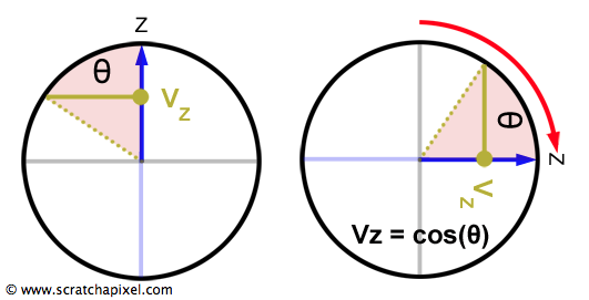
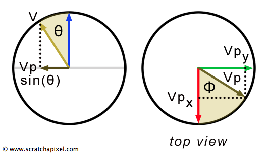
**Figure 6:** Rotating the figure 90 degrees clockwise simplifies understanding that Vz corresponds to $\cos (θ)$ .

Assuming a vector is normalized simplifies its conversion to spherical coordinates. The left-hand image in Figure 6 mirrors the upper image from Figure 4, with a notable difference: the z-axis now serves as the vertical reference. Rotating this diagram by 45 degrees, as shown on the right side of Figure 6, aligns it with the scenario depicted in Figure 1, where x-coordinates were derived using $\cos (θ)$ . This parallel allows us to deduce that Vz is similarly determined by $\cos (θ)$ in this context. Consequently, $θ$ can be accurately calculated through the arccosine of Vz:

V_{z} = \cos (θ) ⟹ θ = acos (V_{z})

In practical terms, within a C++ environment, this translates to:

float theta = acos(Vz);

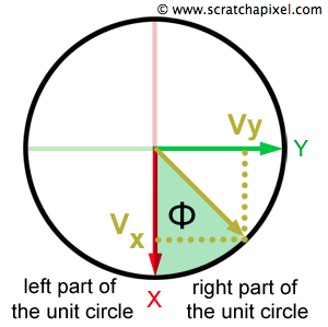
**Figure 7:** Elucidating the calculation of angle $ϕ$ .

Next, we delve into determining $ϕ$ , the horizontal angle. Observing Figure 7, which reflects the lower illustration of Figure 4, the axes are relabeled to x (right axis) and y (forward axis) in red and green, respectively. Recalling our brief overview of trigonometric functions, the tangent of an angle is identified by the ratio of Vy (opposite side) to Vx (adjacent side) within a right-angled triangle. Although one might consider computing $ϕ$ using arccosine similar to $θ$ , it's crucial to remember $ϕ$ 's range extends from 0 to $2 π$ . Employing the tangent and specifically the atan2 function in C++ offers an advantage by factoring in the signs of Vy and Vx. This method yields an angle ranging between 0 to $π$ for vectors on the unit circle's right and between 0 to $- π$ for those on the left. Programmers may need to adjust this outcome to fit within the $[0 : 2 π]$ interval, ensuring universal applicability:

\tan (ϕ) = \frac{V_{y}}{V_{x}} ⟹ ϕ = atan2 (V_{y}, V_{x})

This computation is encapsulated in C++ as:

float phi = atan2(Vy, Vx);

This methodology facilitates the translation of vectors from Cartesian to spherical coordinates, enhancing both the theoretical understanding and practical application of vectors in 3D spaces.

Converting Spherical Coordinates to Cartesian Coordinates

Transitioning from spherical to Cartesian coordinates involves a direct and elegant formula:

x = \cos (ϕ) \sin (θ), y = \sin (ϕ) \sin (θ), z = \cos (θ)

While memorizing this conversion might seem daunting, logical reasoning simplifies its recall. The $z$ component's dependence on $θ$ alone is straightforward, with $V_{z} = \cos (θ)$ demonstrating this relationship. For the $x$ component, consider a scenario where $V$ aligns with the $x$ -axis, specifically at coordinates (1, 0, 0), achievable when $θ = π / 2$ and $ϕ = 0$ . Given that $\sin (π / 2) = 1$ and $\cos (0) = 1$ , it follows that $x = \sin (θ) \cos (ϕ)$ , a deduction also applicable for determining the $y$ component.

Here's a snippet of C++ code to perform the conversion from spherical angles to Cartesian coordinates:

template<typename T>
Vec3<T> sphericalToCartesian(const T &theta, const T &phi) {
    return Vec3<T>(cos(phi) * sin(theta), sin(phi) * sin(theta), cos(theta));
};

This straightforward approach enables the efficient computation of Cartesian coordinates from spherical ones, enhancing the flexibility and utility of geometric transformations in computational applications.

Enhanced Techniques with Trigonometric Functions

Following the explanation of converting between Cartesian and spherical coordinates and their inverse process, we introduce a few practical functions. These functions are invaluable in rendering applications for manipulating vectors across both coordinate systems.

Calculating $θ$ from Cartesian Coordinates

In our discussions, we adopt a left-hand coordinate system where the z-axis signifies the vertical direction for spherical coordinates. As previously discussed, the calculation of $θ$ is given by:

template<typename T>
inline T sphericalTheta(const Vec3<T> &v) {
    return acos(clamp<T>(v[2], -1, 1));
}

It's essential to ensure the input vector is normalized, keeping the z-coordinate within the [-1, 1] range. Employing clamping enhances the robustness of this function.

Deriving $ϕ$ from Cartesian Coordinates

The computation of $ϕ$ presents a different challenge, as the atan function spans the range $[- π, π]$ . To accommodate our needs, we adjust the range to $[0, 2 π]$ as follows:

template<typename T>
inline T sphericalPhi(const Vec3<T> &v) {
    T p = atan2(v[1], v[0]);
    return (p < 0) ? p + 2 * M_PI : p;
}

Simplifying Calculations for Trigonometric Ratios

Beyond calculating angular values, obtaining direct trigonometric ratios such as $\cos (θ)$ , $\sin (θ)$ , $\cos (ϕ)$ , and $\sin (ϕ)$ can be more straightforward:

template<typename T> inline T cosTheta(const Vec3<T> &w) { return w[2]; }

However, determining $\sin (θ)$ necessitates a deeper understanding. Given a unit-length vector, the Pythagorean theorem allows us to assert $V_{x}^{2} + V_{y}^{2} = 1$ . With $V_{x} = \cos (θ)$ and $V_{y} = \sin (θ)$ , it follows that:

\cos (θ)^{2} + \sin (θ)^{2} = 1 ⟹ \sin (θ)^{2} = 1 - \cos (θ)^{2}

To facilitate this calculation, we introduce two functions: one for $\sin (θ)^{2}$ and another for $\sin (θ)$ , leveraging the square root of the former's output.

Projecting Vectors onto the XY Plane

**Figure 8:** Illustrating the projection of vector $v$ onto the xy plane, highlighting the adjustment of its length based on $\sin (θ)$ .

The computation of $\cos (ϕ)$ and $\sin (ϕ)$ becomes nuanced when considering the vector's shadow—or its projection—onto the xy plane. As depicted in Figure 8, a unit-length vector in 3D doesn't necessarily translate to a unit-length projection unless $θ = π / 2$ . This discrepancy arises from the vector's projection, $v_{p}$ , varying in length depending on $θ$ .

**Figure 9:** Demonstrating how the length of $v_{p}$ is determined by $\sin (θ)$ and how its normalized x and y components are utilized to compute $ϕ$ .

The length of the projected vector $v_{p}$ is directly tied to $\sin (θ)$ , as shown in Figure 9. Normalizing $v_{p}$ by dividing its components by $\sin (θ)$ enables the accurate calculation of $\cos (ϕ)$ and $\sin (ϕ)$ through the normalized components:

template<typename T>
inline T cosPhi(const Vec3<T> &w) {
    T sintheta = sinTheta(w);
    if (sintheta == 0) return 1;
    return clamp<T>(w[0] / sintheta, -1, 1);
}

template<typename T>
inline T sinPhi(const Vec3<T> &w) {
    T sintheta = sinTheta(w);
    if (sintheta == 0) return 0;
    return clamp<T>(w[1] / sintheta, -1, 1);
}

This advanced approach to vector manipulation using trigonometric functions and projections enriches the toolbox for rendering, allowing for sophisticated control over vector orientations and interactions within a 3D environment.