Geometry

Matrices

Creating an image with all the 3D elements and the camera fixed at the origin would be quite restrictive. Essentially, matrices are crucial for manipulating objects, lighting, and camera positions within a scene, enabling you to craft your image as desired.

Introduction to Matrices: Simplifying Transformations

In the realm of graphics, matrices are a fundamental component, frequently appearing in the coding of 3D applications. Matrices themselves are not complex; any intimidation they may cause often stems from a lack of understanding regarding their purpose and operation. Let's clarify these aspects.

Previously, we discussed the capability to shift or rotate points through linear operations. For instance, we demonstrated that moving a point could be achieved by adjusting its coordinate values. Similarly, we illustrated that a vector's rotation could be managed using trigonometric functions. To put it succinctly (without delving into a formal mathematical explanation), matrices amalgamate these transformations—scaling, rotating, and translating—into a unified entity. Applying a matrix to a point or vector effects a transformation, encompassing any mix of scaling, rotation, and translation. For instance, one can craft a matrix that rotates a point 90 degrees around the x-axis, enlarges it twofold along the z-axis (applying a scale of (1, 1, 2)), and then shifts it by (-2, 3, 1). While it's feasible to execute these transformations sequentially on a point, doing so could necessitate extensive coding:

Vec3f translate(Vec3f P, Vec3f translateValue) { ... }
Vec3f scale(Vec3f P, Vec3f scaleValue) { ... }
Vec3f rotate(Vec3f P, Vec3f axis, float angle) { ... }
...
Vec3f P = Vec3f(1, 1, 1);
Vec3f translateVal(-1, 2, 4);
Vec3f scaleVal(1, 1, 2);
Vec3f axis(1, 0, 0);
float angle = 90;
Vec3f Pt;
Pt = translate(P, translateVal);  // First, translate P
Pt = scale(Pt, scaleVal);         // Next, scale the result
Pt = rotateValue(Pt, axis, angle); // Finally, rotate the point

This process can be streamlined considerably with matrices, allowing us to write:

Matrix4f M(...);  // Initialize the matrix for translation, rotation, and scale.
Vec3f P = Vec3f(1, 1, 1);
Vec3f Ptransformed = P * M;  // Execute translation, rotation, and scale in one step.

By multiplying a point with a matrix (M), we achieve a transformation of P that incorporates translation, rotation, and scaling all at once. This demonstrates the utility of matrices in the graphics pipeline and their benefits. In this particular instance, we've illustrated that matrices can unify the three fundamental geometric transformations (scale, translation, rotation) in an efficient, straightforward, and compact manner. Our next goal is to delve into how and why this integration is effective, although it will require several chapters to fully explore.

Understanding Matrices

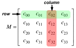
What exactly are matrices, and what secrets do they unlock? Rather than delving into an abstract mathematical definition, we'll begin with practical examples of matrices. Once we've explored a few tangible instances, extending these concepts to a more generic or mathematical form will become simpler. If you've encountered matrices in computer graphics literature, you may have noticed they often appear as a two-dimensional array of numbers. This array is described by the notation m x n, where m and n denote the array's dimensions. Here, m and n correspond to the number of rows and columns in the matrix, with rows running horizontally and columns vertically. Here's an example of a [3x5] matrix:

In this context, we refer to the elements of the matrix as coefficients, and they are often indexed using the subscripts i (row) and j (column). Matrices are usually denoted with capital letters (M, A, B, etc.).

\(M_{ij}\) indicates the coefficient at the intersection of row i and column j.

For simplicity, especially in computer graphics (CG), we often focus on square matrices, where the number of rows and columns are equal, typically 3x3 or 4x4. These square matrices play a pivotal role in CG, though it's important to note that matrices can have any dimensionality (e.g., 3x1, 6x6, 4x2). However, our discussion will mainly revolve around 3x3 and 4x4 matrices for their prevalent use in CG.

Examples of square matrices include a [3x3] \(\begin{bmatrix} 7&4&3\\ 2&0&3\\ 3&9&1\\ \end{bmatrix}\) and a [4x4] \(\begin{bmatrix} 7&1&4&3\\ 2&0&0&3\\ 3&1&9&1\\ 6&6&5&4\\ \end{bmatrix}\) matrix.

Below is an example of how a 4x4 matrix class could be implemented in C++, using templates for flexibility with different data types:

template<typename T> 
class Matrix44 
{ 
public: 
    Matrix44() {} 
    const T* operator [] (uint8_t i) const { return m[i]; } 
    T* operator [] (uint8_t i) { return m[i]; } 
    // Initialize matrix coefficients to the identity matrix
    T m[4][4] = {{1,0,0,0},{0,1,0,0},{0,0,1,0},{0,0,0,1}}; 
}; 
 
typedef Matrix44<float> Matrix44f; 

const T* operator [] (uint8_t i) const { return m[i]; } 
T* operator [] (uint8_t i) { return m[i]; } 

Matrix44f mat; 
mat.m[0][3] = 1.f; 

Matrix44f mat; 
mat[0][3] = 1.f; 

Matrix Multiplication

Matrices can be multiplied together, a fundamental operation that underpins the transformation of points or vectors through matrices. The outcome of this operation, known as the matrix product, is a new matrix:

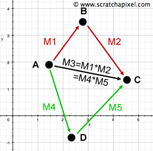
Recall our initial discussion, where we introduced the idea that a matrix encapsulates a set of linear transformations (scale, rotation, translation) that can be applied to points and vectors. While we've yet to delve into the workings of this concept, it's crucial to understand now that matrix multiplication allows us to merge the effects of two matrices into a single matrix. This means that the transformations applied by matrices M1 and M2 to a point or vector can be combined into a single matrix, M3. For instance, if you need to transform a point from A to B with matrix M1 and then from B to C with matrix M2, multiplying M1 by M2 yields a matrix M3 that directly transforms A to C. The resultant matrix from the multiplication of two matrices serves the same function as the individual matrices. It's worth noting that if there are two other matrices, M4 and M5, that transform A to D and D to C respectively, then the multiplication of M4 and M5 will also produce M3, highlighting that there is a unique matrix for each specific transformation.

There's a specific rule about matrix multiplication which, while not crucial when working exclusively with 4x4 matrices, is worth knowing for a broader understanding of the subject. This rule states that two matrices, M1 and M2, can only be multiplied if the number of columns in M1 is equal to the number of rows in M2. This means that matrices sized m x p and p x n can be multiplied to produce a matrix of dimensions m x n. Conversely, matrices sized p x m and n x p cannot be multiplied if m and n are unequal. For example, a 4x2 matrix can be multiplied with a 2x3 matrix to produce a 4x3 matrix. When multiplying two 4x4 matrices, the result is another 4x4 matrix, which aligns with our primary focus and simplifies our discussion.

Let's explore the process of multiplying two matrices, focusing on how the coefficients of the resultant matrix are calculated. This process involves matching the row from the first matrix and the column from the second matrix, then multiplying and summing the corresponding elements. Consider finding the coefficient M3(1,2) in matrix M3. If we take the second row of M1 and the third column of M2 (both 4x4 matrices), we obtain two sequences of numbers. These are then multiplied pairwise and summed to compute the coefficient M3(1,2) as follows:

This method is applied to compute all coefficients of M3, utilizing the respective row and column indices to select the corresponding coefficients in M1 and M2. Once identified, these coefficients are multiplied and summed to determine the value of M3(i,j):

Here's how this multiplication operation can be implemented in C++, using a 4x4 matrix defined as a two-dimensional array of floats:

Matrix44 operator * (const Matrix44& rhs) const
{
    Matrix44 mult;
    for (uint8_t i = 0; i < 4; ++i) {
        for (uint8_t j = 0; j < 4; ++j) {
            mult[i][j] = m[i][0] * rhs[0][j] +
                         m[i][1] * rhs[1][j] +
                         m[i][2] * rhs[2][j] +
                         m[i][3] * rhs[3][j];
        }
    }

    return mult;
}

Understanding matrix multiplication reveals that the operation is not commutative—the order of multiplication matters, and thus M1*M2 will yield a different result from M2*M1.

Summary

In summary, although we have not yet delved into the specifics of how and why matrices function, rest assured that these critical details will be covered in the forthcoming chapter. From our current discussion, the key takeaway should be that a matrix represents a two-dimensional array of numbers, with its dimensions indicated by \(m \times n\), where \(m\) stands for the number of rows and \(n\) for the number of columns. It's crucial to understand that matrices can only be multiplied if the number of columns in the left matrix matches the number of rows in the right matrix. For example, matrices of dimensions \(m \times p\) and \(p \times n\) are compatible for multiplication. The product of such multiplication effectively merges the transformations represented by the two matrices involved. For instance, if matrix M1 effects a transformation from point A to B, and matrix M2 from B to C, then their product, M3, will transform a point directly from A to C. Additionally, we've explored the methodology for calculating the coefficients of a resulting matrix post-multiplication. Another vital concept to grasp is that matrix multiplication is inherently non-commutative, meaning the sequence of multiplication significantly impacts the outcome. Thus, when troubleshooting code issues, verifying the multiplication sequence of matrices is a prudent step.