Geometry

Transforming Normals

Reading time: 10 mins.

Understanding Surface Normals

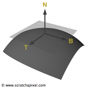
**Figure 1:** The tangent (T) and bi-tangent (B) lie on the plane tangent at point P. The cross product of T and B yields the surface normal N. It's important to note that T, B, and N are orthogonal to each other, forming a Cartesian coordinate system.

Previously introduced in the opening chapter of this series, the concept of a surface normal is revisited here for a more in-depth discussion. A surface normal at a point P on a surface is defined as a vector that is perpendicular to the tangent plane at that point. The forthcoming sections on geometric primitives will detail the computation of normals. However, for now, it suffices to understand that if the tangent T and bi-tangent B at point P are known—these vectors defining the plane tangent to the surface at P—then the surface normal at P can be derived through a straightforward cross-product:

$$N = T \times B$$

The cross-product operation is characterized by its anticommutative property, which implies that exchanging any two operands reverses the result's sign. Hence, $T \times B = N$ and $B \times T = -N$. This characteristic necessitates careful consideration when calculating the normal to ensure it points outward from the surface, a crucial aspect for shading applications, which will be elaborated upon in subsequent lessons.

Transforming Normals: A Detailed Examination

**Figure 2:** a) Illustrates the normal to line AB in blue. b) Shows the effect of non-uniform scaling on AB and its normal, resulting in the transformed normal no longer being perpendicular to A'B'. c) Demonstrates that transforming the normal with the transpose of the inverse matrix maintains orthogonality with A'B'.

Why treat normals distinctively from vectors? This differentiation arises from the challenge of transforming normals in the same manner as points and vectors, which isn't always appropriate, especially under non-uniform scaling. For instance, considering a 2D scenario with a line intersecting points A=(0, 1, 0) and B=(1, 0, 0), drawing a line from the origin to (1, 1, 0) yields a line perpendicular to our plane, representing our normal N. Ignoring normalization for simplicity, let's apply a non-uniform scale to this setup using a transformation matrix:

$$ M= \begin{bmatrix} 2&0&0&0\\ 0&1&0&0\\ 0&0&1&0\\ 0&0&0&1 \end{bmatrix} $$

This scaling transforms A and B to A'=(0, 1, 0) and B'=(2, 0, 0), respectively. Applying the same transformation to N yields N'=(2, 1, 0), visibly altering its perpendicularity to the line through A' and B'.

When transforming normals in computer graphics, especially under non-uniform scaling, we need to use the transpose of the inverse of the transformation matrix, $M^{-1T}$. This method ensures that normals remain correctly perpendicular to the surface after transformation.

Here's a breakdown of this concept:

Rotations and Orthogonal Matrices

First, normals, being direction vectors, should be transformed differently than points to preserve their geometric relationship with surfaces. For rotations, represented by orthogonal matrices (where a matrix $Q$ satisfies $Q^T = Q^{-1}$), applying $M^{-1T}$ to normals does not alter their correct orientation post-transformation. This is because the transpose of the inverse of a pure rotation matrix effectively results in the original rotation matrix itself, due to the property of orthogonal matrices. Thus, for rotations alone, the process of using $M^{-1T}$ seems redundant but is indeed valid.

Non-Uniform Scaling and Combined Transformations

The complication arises with non-uniform scaling, where different axes of an object are scaled by different amounts. Applying the same transformation matrix to normals as we do for points or direction vectors can lead to incorrect orientations, as normals may no longer remain perpendicular to the surface.

A reader might question, "If a matrix $M$ encodes both rotation and scaling, does it still maintain orthogonality?" The answer is nuanced. A matrix that combines rotations and non-uniform scaling is not orthogonal due to the scaling component. However, we can conceptually decompose such a matrix into two separate matrices: one for rotation ($R$), which is orthogonal, and one for scaling ($S$).

$$M = R * S$$

This decomposition helps us understand that the issue with transforming normals correctly lies not with the rotation part ($R$) but with the scaling part ($S$). Since we've already established that $R^{-1T} = R$ for rotation matrices, the challenge remains with how to handle the scaling matrix $S$ effectively.

Addressing the Scaling Issue

The key insight is that transforming normals correctly under non-uniform scaling requires adjusting for the scale differently. The operation $M^{-1T}$ effectively addresses this by modifying the scale factors appropriately. For the scaling matrix $S$, taking its inverse ($S^{-1}$) adjusts the scale factors in the opposite direction (e.g., a scale factor of 2 becomes $1/2$), and transposing this inverse ($S^{-1T}$) does not alter its effect on scale factors since transposition does not change the diagonal elements of $S$.

$$ M^{-1T}= \begin{bmatrix} 1 \over 2&0&0&0\\ 0&1&0&0\\ 0&0&1&0\\ 0&0&0&1 \end{bmatrix} $$

Therefore, when we apply $M^{-1T}$ to a normal, we are effectively applying $R$ for rotation, which is appropriate, and correctly adjusting the scale factors via $S^{-1}$ to ensure the normal remains properly oriented relative to the surface post-transformation.

In summary, the use of the transpose of the inverse matrix, $M^{-1T}$, for transforming normals is a nuanced approach that correctly addresses both rotation and non-uniform scaling. By decomposing the transformation into its rotational and scaling components, we can see that the approach effectively maintains the orthogonality of normals to surfaces, ensuring accurate geometric and shading calculations in computer graphics.

While it's feasible to derive normals from transformed vertices, this method is unsuitable for shapes like spheres transformed into ellipsoids through non-uniform scaling. Directly applying the transformation matrix to normals in such cases does not yield correct orientations. However, if derivatives (tangent and bitangent) at a surface point are known, a correctly transformed normal can be computed from these derivatives, regardless of the shape. This approach is adopted in our basic renderer, but when derivatives are unavailable, utilizing the transpose of the inverse matrix remains the universal solution.

Mathematical Justification for Transposing the Inverse in Normal Transformations

When considering the dot product between two orthogonal vectors, $v$ and $n$, where $v$ lies within the tangent plane at point P and $n$ is the normal to this plane, the dot product equals zero because the vectors are perpendicular:

$$ v \cdot n = 0 $$

This mathematical principle can be represented in the context of matrix operations. To do this, we express the dot product as a matrix multiplication where $v$ is treated as a [1x3] matrix (row vector) and $n$ as a [3x1] matrix (column vector). This arrangement is essential for performing matrix multiplication, as the dimensions align correctly ([1x3] multiplied by [3x1] yields a [1x1] matrix, or a scalar value). Here's the transformation of $v$ and $n$ into matrix form and the subsequent multiplication:

$$ \begin{pmatrix} v_x & v_y & v_z \end{pmatrix} * \begin{pmatrix} n_x\\ n_y\\ n_z \end{pmatrix} = v * n^T $$

In this equation, $n^T$ represents the transpose of the normal vector $n$, converting it from a [1x3] row vector to a [3x1] column vector, suitable for multiplication with $v$. The result of this operation, $v * n^T$, should be zero, mirroring the outcome of their dot product, because the fundamental geometric relationship between $v$ and $n$ remains unchanged by this representation. This approach bridges the concept of dot products in vector algebra with matrix multiplication in linear algebra, demonstrating that orthogonal vectors yield a zero product whether considered as vectors or matrices.

Considering $M$ as the transformation matrix and $I$ as the identity matrix, we know that $M * M^{-1} = I$, implying that inserting $M^{-1} * M$ within $v * n^T$ has no effect. However, rearranging the terms gives:

$$v * n^T = (v*M) * (n*M^{-1T})^T$$

Here, $v*M$ represents the transformed vector $v'$, applicable for vectors within the plane tangent to P. Rearranging to $n*M^{-1T}$ accounts for transforming the normal, necessitating the transpose of the inverse matrix for correctness:

$$v * n^T =v' * n'^T$$

This equation must hold true as the dot product between $v$ and $n$ remains invariant under linear transformations. Therefore, if $(n * M^{-1T})^T=n'^T$, it confirms that $n'=n * M^{-1T}$, validating the approach for transforming normals to maintain their perpendicular orientation to the surface after transformation.

$$v \cdot n = v * n^T = v_x * n_x + v_y * n_y + v_z * n_z = 0$$

Assuming $v$ and $n$ are orthogonal.

When we incorporate a transformation matrix $M$ into the equation relating $v$ and $n$, the normal and tangent vector at point P, we initially introduce an intermediate step to demonstrate how transformations affect these vectors:

$$v * n^T = v * M * M^{-1} * n^T$$

Here, $M$ represents the matrix used to transform point P, and $I$ symbolizes the identity matrix. The multiplication of a matrix by its inverse ($M * M^{-1}$) yields the identity matrix ($I$), indicating that inserting $M^{-1} * M$ effectively makes no change to the original relationship between $v$ and $n$. This operation might seem redundant at first, but it sets the stage for re-arranging and further understanding the transformation process:

$$v * n^T = (v*M) * (n*M^{-1T})^T$$

When examining the term $v*M$, it signifies the vector $v$ after being transformed by the matrix $M$, which we denote as $v'$. This transformation is specifically relevant for vectors that are tangent to the surface at point P. We've previously discussed that applying the transformation matrix $M$ to vectors is straightforward and does not pose issues as it does with normals. Therefore, when we apply $M$ to $v$, a vector tangent to P, we obtain $v'$, another vector that remains tangent to the transformed surface. This is expressed as:

$$v' = v * M$$

This process illustrates that $v'$ is the result of transforming $v$ by $M$, ensuring that $v'$ maintains its tangential property relative to the surface after transformation.

Concerning the second term $n*M^{-1T}$, we've rearranged this expression by moving $M^{-1}$ to follow $n^T$, necessitating the application of a transpose to $M^{-1}$, thus writing it as $M^{-1T}$. This step adheres to the algebraic principle where the multiplication order of matrices can be adjusted if we transpose one of them, akin to the example $M_A \times M_B = M_B^T \times M_A$, which helps us maintain the logical flow of the transformation.

Finally we have:

$$v * n^T = v' * n'^T$$

This equation asserts that the relationship defined by the dot product between vector $v$ and normal $n$, which originally equals zero due to their orthogonal nature, remains unchanged after transformation. This invariance of the dot product under linear transformations is a fundamental property we rely on. To preserve this relationship, the transformed vector $v'$ is obtained by applying the transformation matrix $M$ to $v$, as previously discussed.

Now, focusing on the normal $n$, when we apply the transformation $M^{-1T}$ to $n$ and then transpose the result, we aim to maintain the orthogonality between $v'$ and the transformed normal $n'$. If the operation $(n * M^{-1T})^T$ yields $n'^T$, it logically follows that the transformed normal $n'$ is correctly obtained by applying $n * M^{-1T}$.