Color Space
Reading time: 30 mins.Remember that this lesson is only an introduction to the topic of colors. It gives enough information for the reader to understand the main concepts and techniques used to represent and manipulate colors in computer graphics (at least enough to render images). The goal of this lesson is not to make an exhaustive list of colors spaces.
In the first chapter of this lesson we have presented the most important concepts regarding light and colors. The color of an object or the color of a light, can be seen as the result of many different light colors from the visible spectrum mixed together. The light colors a particular light is made of, is described by its spectral power distribution. The problem with this representation, is that human eyes can not directly perceive SPDs. We have also described in the previous chapter how the eyes are based on a trichomatic color vision system and also how we perceive colors in normal lighting environments differently than in dark lighting conditions. Therefore, to represent colors, we need to convert SPDs into another representation which is better suited for our trichomatic vision. We call such representations color models or color spaces (you will understand why in this chapter). Many color models exist but in this lesson we will present the CIE XYZ color model which is the foundation of all color models as well as the RGB model which is a popular model in computer graphics. As a short answer, you can see a color model as a technique of mapping the values from a SPD to three values (the tristimulus values) which can more directly relate to the way our eyes perceive colors.
It is important while reading this chapter to keep in mind the distinction between the notion of color and value or lightness of a color. The color of a color (so to speak) is called hue. It is sometimes referred to as chromaticity which defines the quality of a color independently from its lightness.
What is a Color Space?

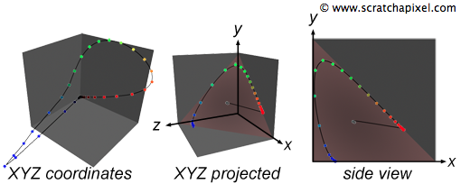
A color space is a model which can be used to represent as many colors as our vision system can possibly perceive (however, most often, they can only represent a subset of these colors). By colors we usually refer to the colors that the human visual system can perceive (which is the main advantage of the XYZ color model: it tries to stick the human vision system's response to colors) and the various colors which can be obtained by all the possible combinations of all the light colors from the visible spectrum (remember that the human vision system is perceptual). The range of possible colors that can be represented by a particular system is called the gamut. A color space in its most simplistic form, can be seen as the combination of three primary colors (reg, green blue) in a color additive system. Adding any of these colors to each other can produce a wide range of colors (this is the base of the RGB color model). The gamut of the CIE xyY color space for example, has a horseshoe shape as showed in Figure 1 (colors are plotted using the CIE xyY color space where xy represents the color's chromaticiy. This model is detailed further down). This shape varies depending on the color space used. Note that somewhere on this gamut is a particular region where the colors converge to an impression of white. This is called the gamut's white point. Naturally, what we are interested in are really the colors that the human eye can perceive. Any other color space that do not make it possible to represent all the colors we can see, is more limited or more restrictive than any other system that can represent all possible perceivable colors. In fact, most existing color space models are limited in their capacity to cover the full gamut. But what do we call a full gamut anyway? It is a gamut that would represent all the colors than the human eye can perceive. In fact, technically, this gamut is called the gamut of human vision and the XYZ color space model was designed with this particular goal in mind. You might still wonder though why it is called a space. To represent colors a minimum of three variables (XYZ, RGB, HSV, etc.) are needed like for 3D points and the set of all possible values these variables can take on the range over which they are defined can be drawn in 3D space and define a volume or space (this will be more easily understandable when we will talk about the RGB color model).
CIE XYZ and xyY Color Models
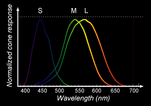
Even though inaccurate, we can start from the assumption that the three main types of cones responsible for color vision we can find in the eye, are sensitive to blue (S(-hort) cone), green (M(-edium) cones) and red (L(-ong) cones) light (it is inaccurate because recent measurements showed that the peak of sensitivity for L cones is more around yellow than red. S and M cones are themselves not perfectly centered on blue and green as you can see in Figure 2. Also it is important to remember that the distribution of cones and therefore these curves vary from person to person. However this simplification led the CIE to conduct an experiment in the early 1930s based on the idea that any color (in an additive color model) can be represented by a combination of red, green and blue light which each type of cones in the eyes are sensitive to. The experiment consisted in asking a large number of people to recreate colors that were showed to them on a screen by combining various amount of pure red, green and blue light. Because cone cells are mainly focused towards the centre of the retina, their vision was restricted to a 2 degrees angle, to avoid their perception of color to be biased by the contribution of the rod cells which as we mentioned in the previous chapter, are helping us to see things in low light conditions but without a sense of colors.
They also realized while doing this experiment, that some colors could be obtained using different combinations of primary red, green and blue light. This is called metamerism.
From the result of this experiment, they plotted the amount of primary red, green and blue light needed to represent each color from the visible spectrum. The result of this experiment gives three curves known as the CIE standard observer color matching functions (they can be referred to in the literature as the CIE 1931 2° standard observer):
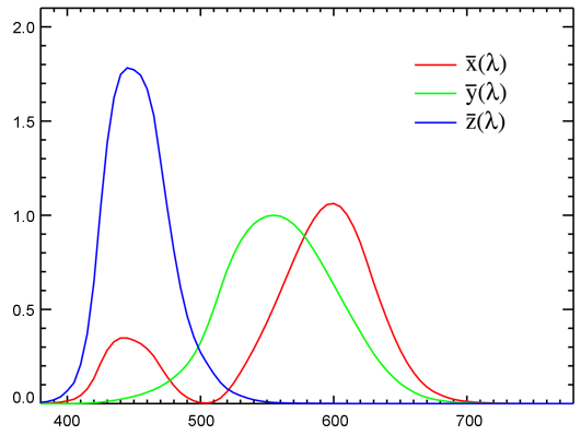
One important thing to notice is that the green curve strangely corresponds to the luminosity function which as we mentioned in the previous chapter represents the sensitivity of the human eye to brightness. We started from a spectrum which we know we can't see and we now have three more curves. How can that possibly make things simpler? From these curves, we can now convert the spectrum into three values which we call X, Y, Z using the following formulas:
Where
The symbol
Usually the spectrum and the color-matching functions are discrete (defined by a series of samples); they are not represented as a function defining a continuous curve, but as a series of discrete samples or points which we can "connect" to each other to make a curve. If the data color matching functions, the spectrum data cover the same range of wavelengths (for example from 380 to 780) and the number of points is the same (we have one sample every 5 nm starting at 380 nm and finishing at 780 nm which makes 81 samples), then we can then compute XYZ using the following code (we will explain this code later in this chapter):
void SpectrumToXYZ(int colorIndex, float XYZ[])
{
    float Ysum = 0;
    for (int i = 0; i < 81; ++i) {
        XYZ[0] += colorMatchingFunc[i][0] * spectralData[colorIndex][i];
        XYZ[1] += colorMatchingFunc[i][1] * spectralData[colorIndex][i];
        XYZ[2] += colorMatchingFunc[i][2] * spectralData[colorIndex][i];
        Ysum += colorMatchingFunc[i][1];
    }
    XYZ[0] *= 1 / Ysum;
    XYZ[1] *= 1 / Ysum;
    XYZ[2] *= 1 / Ysum;
}
In this example the spectral data varies from 350 to 750 nm and is sampled every 5 nm however you can either use more precise data (one sample every 1 nm) or less (one sample for each 10 nm) and reduce the range as well (for instance from 400 to 750). Spectrum data for materials or lights are hard to find so this choice is more a matter of adapting our code to what's available. Using less data means computing XYZ quicker and using more data means a more precise result (but also longer computation time). You can better understand now why spectrum renderer are usually slower than renderers using the more basic RGB color system.
But how can these three values be more meaningful to us than the spectrum itself? As such they are not really useful indeed because XYZ colors can't be displayed on a computer screen. To display XYZ colors we have to convert them to a RGB colors first using a technique which we are going to describe soon. The main advantage of the XYZ color space though, is that it is the best of all the existing systems to represent all the colors that we can see. Of all the existing color spaces, it is the model that can best represent all the colors that the human vision can perceive (in other words the gamuts of over color spaces are usually smaller or contained within the gamut of the XYZ color space). As such it is probably the best system for storing color information and is still considered today as the gold standard. Before we can learn how to convert an XYZ color to an RGB color we will first introduce the RGB color space. However before we conclude this part of the lesson, lets just speak about the meaning of the X Y and Z values themselves. In fact, as we have already mentioned the Y color matching function is really close to the luminosity function. As such some people like to see the Y value from the XYZ tuple as expressing the brightness of a color. The values of an XYZ color can't really be directly used as RGB values however they can also certainly give an indication of how much red, green and blue a color is made of.
To integrate the spectral data of a light source (the technique is the same for materials), we need to sum up all the data from the spectrum multiplied by the distance between two consecutive samples. The resulting number defines the power of the light source (which can either be expressed in Joules or in Watts). This concept if important because many renderers don't deal with spectrum data directly but relies on the user to specify the power or intensity of light sources. Being able to compute this power can be useful to set our light sources with physically meaningful data (note that from this spectrum we can also compute an XYZ value which we then convert to RGB). Mathematically, this integration takes the following form: $Power = \Phi_e = \int_{\lambda_0}^{\lambda_1} S_e(\lambda) d\lambda$ Where
The xyY Color Space
The xyY color space is derived from the XYZ and we will just mention it briefly as it used to draw images of the color space's gamut such as in Figure 1. We have mentioned before that it was important to make the separate the concept of chromaticity which defined how colorful a color is from the concept of a color's brightness. A typical example is the color white which has the same chromaticity than a gray color but doesn't have the same brightness than white. The xyY color space was developed in order to be able to separate these two properties and use only two components (x and y) to encode the color's chromaticity and keep the Y value from the XYZ tristimulus values to encode the color's brightness or value. The idea is simple. It consists of normalizing the three components of a XYZ color by the sum of these components:
Once normalized, the values of the resulting x y and z components sum up to 1. Therefore we can find the value of any of the components if we know the values of the other two. For example with z we can write:
RGB Color Space
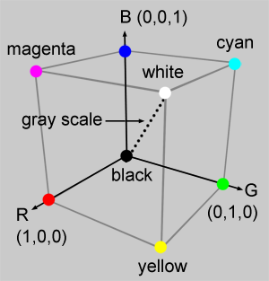
The idea of the RGB color space is really to stick to the principle of human vision and represent colors as a simple sum of any quantities (from 0 to 1) of the primary colors (red, green and blue). As such it can be represented as a simple cube (Figure 4) where three of the vertices represent the primary colors. Moving in one direction along the vertices of this cube results in blending two of the primary colors together which leads when we reach the vertex of the cube opposite to two primary colors, to a secondary color (either cyan, magenta or yellow). Two of the cube vertices are special as they correspond to white (when the three primary colors are mixed up together in full amount) and black (absence of any of the three primary colors). These vertices defines a diagonal along which all the colors are gray (gray scale). Note here that we speak of color in terms of their chromaticity, not in terms of their possible brightness or value.
Red |
Green |
Blue |
White Point (E) |
|
|---|---|---|---|---|
x |
0.7347 |
0.2738 |
0.1666 |
0.31271 |
y |
0.2653 |
0.7174 |
0.0089 |
0.32902 |
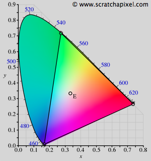
The RGB color space is one of the most basic color spaces in existence which is probably a reason for its popularity. It is also simple to understand and visualize (as with the example of the cube). However its gamut is much more limited than that of the XYZ color space as showed in Figure 5. It can be represented as a triangle contained within the horseshoe shape of the XYZ's gamut where each of the triangle vertices represents a primary color expressed with regard to the XYZ color space (more precisely these coordinates are expressed in the xyY color space which we have used before to draw the horseshoe shaped XYZ gamut). The coordinates of the red, green and blue RGB colors expressed with regards to the xyY color space are summarized in the table on the right. Note that the coordinates of the white point are also defined (the white point of a particular color space might vary depending on the viewing conditions it was designed for). In the case of CIE RGB, the white point is defined as being the illuminant E which is, like the illuminant D65 which we talked about in the previous chapter, a predefined CIE illuminant that has the property of having a constant SPD across the visible spectrum (an illuminant that gives equal weight to all wavelengths). We can plot these coordinates on our existing horseshoe shape and draw lines to connect the dots. You can see that it defines a triangle. All colors contained within the limits of this triangle are the color which we can represent if we use the RGB color space. You can also see that the colors that we can represent with this model, are much more limited than those we can define using the XYZ color space (see figure 5).
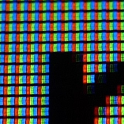
Most computer screens technology is based on a system similar to the RGB color model. Each pixel on the screen is made of three small lights, one red, one green and one blue, which contribution sums up to white when they are all three turned on at the same time (when you look at the screen up close you can distinguish the three color but from the distance they blend into white). However we will show in the next chapter that computer screens can also manipulate colors in a way that we are not always very much aware of.
Finally lets mention that the RGB color model is not the only type of RGB color space in existence. Several other models based on the same principle as the RGB color space have been proposed to enhance the original model or as an attempt to address particular issues. For example the sRGB color model applies a gamma correction (which we will explain in the next chapter) to the original RGB values as a way of better representing the human vision response to variations of brightness (which is non linear). Such models are said to be non linear because they modify the original RGB or XYZ linear tristimulus values into non linear values. This will be fully explained in the next chapter. In this chapter though we will stick to linear color spaces such as XYZ and RGB.
The rule of thumb when rendering images with a 3D renderer is that all input and output colors should be expressed with regard to a linear color space such as XYZ or RGB. Colors expressed in a non-linear color space (such as sRGB) should be converted back to RGB before being used by a renderer. Read the next chapter to learn more about gamma correction and non-linear color spaces.
Converting XYZ to RGB
You can read the lesson on geometry to better understand how matrices work and then come back to this part of the lesson later if you wish. Using XYZ or spectral data in a renderer is an advanced topic and we won't be using this technique in the basic version of the renderer. In this introduction on colors, we won't spend much time explaining where the numbers for converting a XYZ to an RGB color come from, however you will find a lesson on this matter in the advanced 2D section.
The conversion fron XYZ to RGB can be done using a [3x3] matrix. Remember from the beginning of this chapter that colors defined in a particular color space are usually defined by three coordinates (that is at least the case of the RGB and XYZ color spaces) which can be plotted in 3D space. And when all the colors from the gamut that one particular color space can represent, are plotted in 3D space, they define a volume (a cube in the case of the RGB model for example as illustrated in figure 4). The conversion of a color defined in one color space to another color space can simply be seen as moving a point in 3D space from one position to another. And generally such linear transformation is best handled by matrices. Keep in mind that this transformation do not change the color itself. It is used to express the same color in different color spaces. Not all color space transformations can be handled by [3x3] matrices. Some may require more complex mathematical formulas such as for instance a transform from the RGB to the HSV (hue-saturation-value) color space (check the 2D section for more information on color spaces).
Matrix multiplication can be thought of as a linear transformation (see the lesson on Geometry for more information on linear operator or transformation using matrices). In other words (when applied to the fied of color spaces) matrices can only be used to transform between linear color spaces. This detail might sound abstract if you don't know yet about the difference between linear and non-linear space (such as sRGB for instance) which we will talk about in the next chapter. However readers aware of the difference should keep in mind that [3x3] matrices can't be used to convert between non linear and linear color space (or vice versa). Any non linear color space must be converted to a linear color space before such transform is applied.
The following code shows a method to convert a color defined in XYZ to the RGB color space using a [3x3] matrix (don't worry so much about where the numbers come from. Generally it is good enough to find these matrices on the web and use them directly in your program):
void SpectrumToXYZ(int colorIndex, float XYZ[])
{
    float Ysum = 0;
    for (int i = 0; i < 81; ++i) {
        XYZ[0] += colorMatchingFunc[i][0] * spectralData[colorIndex][i];
        XYZ[1] += colorMatchingFunc[i][1] * spectralData[colorIndex][i];
        XYZ[2] += colorMatchingFunc[i][2] * spectralData[colorIndex][i];
        Ysum += colorMatchingFunc[i][1];
    }
    XYZ[0] *= 1 / Ysum;
    XYZ[1] *= 1 / Ysum;
    XYZ[2] *= 1 / Ysum;
}

float XYZ2RGB[3][3] =
{
    { 2.3706743, -0.9000405, -0.4706338},
    {-0.5138850,  1.4253036,  0.0885814},
    { 0.0052982, -0.0146949,  1.0093968}
};

void convertXYZtoRGB(float XYZ[], float rgb[], const float XYZ2RGB[3][3])
{
    rgb[0] = XYZ2RGB[0][0] * XYZ[0] + XYZ2RGB[0][1] * XYZ[1] + XYZ2RGB[0][2] * XYZ[2];
    rgb[1] = XYZ2RGB[1][0] * XYZ[0] + XYZ2RGB[1][1] * XYZ[1] + XYZ2RGB[1][2] * XYZ[2];
    rgb[2] = XYZ2RGB[2][0] * XYZ[0] + XYZ2RGB[2][1] * XYZ[1] + XYZ2RGB[2][2] * XYZ[2];
}

... convertXYZtoRGB(XYZ, rgb, XYZ2RGB); ...
Exercise: The Macbeth Chart
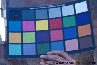
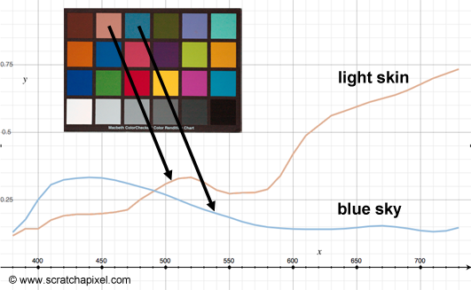
What is a Macbeth chart? A Macbeth chart is a flat piece of cardboard on which you will find a selection of twenty four colored patches (six columns and four rows). These colors are always the same and corresponds to the average reflectance of typical materials which are often photographed, such as human skin, sky and foliage. These colors no matter where the Macbeth is produced should always be the same as the chart is used as a reference against which the exposition and color settings of the camera can be tweaked. Because the colors of these twenty four patchs are always the same and produced under controled conditions, we can use a spectrophometer to measure the spectral power distribution (SPD) of each one of these squares (under constant and controlled ligthing conditions). You can see the spectral curves of two colors (light skin and blue sky) from the Macbeth chart in Figure 9. The Macbeth chart spectral data can easily be found on the web in the form of a table, composed on 24 entries where each entry corresponds to one of the colors on the chart. Depending on the precision of the measurement, the color's SPD can be sampled every 1, 2, 5 or 10 nanometers in a range which boundaries can change but has to fit within the visible spectrum (generally from 380 to 780 nm).
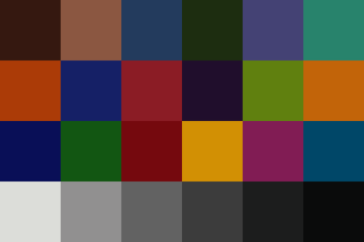
The data we will use in our exercise is sampled every 5 nm from 380 to 780 nm. We also need the CIE color matching functions which you can download from the CIE website itself. We will be using this data to compute a XYZ value for each patch of the Macbeth chart using the code given above. For each component of the XYZ tuple, we need to multiply the spectral data of a patch with the corresponding sample from the corresponding color matching function (either
For this particular exercise though, we use spectral reflectance curves. They define the properties of a certain object to reflect (or absorb) light of a certain wavelength. However, we see objects because they are illuminated by lights which have their own spectral emission curve (or their own color temperature). The color of an object under sunlight for instance might seem different than when observed under the illumination of an artificial light source (a street light). Thus, ideally, to visualize the spectral reflectance curves of the Macbeth chart as colors, we also need to simulate under which lighting conditions we want to look at these colors. For doing so, what we need is to multiply the reflectance data of each given color by the spectral profile of the light under which we want to look at these colors as well as the CIE color matching functions when they are converted to XYZ values. Remember from the previous chapter that the spectral profile of a light is what we call an illuminant.
A standard illuminant is a theoretical source of visible light with a profile (its spectral power distribution) which is published.
We can re-write the equations for computing XYZ as follows:
Where
D65 corresponds roughly to a midday sun in Western Europe / Northern Europe, hence it is also called a daylight illuminant.

Finally, to visualise our results, we will save the colors to an image file (to learn how to save an image file to disk, check the lesson on Digital Images: from File to Screen). The complete code for this exercice is available in the Soure Code chapter. The result of the program is showed in Figure 8. Compare this result to the photograph of the real Macbeth chart (Figure 7). For this introduction on colors, we just wanted to give a simple example to better help readers understand the basic (and simple) process of converting spectral data (which can't be displayed on the screen) to RGB values (which can be displayed on the screen).
To keep the program short, we have truncated the spectral data (but they can be found in the provided source code). The first set of data (lines 3 to 6) are the color machine functions data. The first column or number (line 4) indicates the wavelength the data corresponds to. The following columns (2, 3 and 4) correspond to the
static const int numBins = 81;
const float colorMatchingFunc[numBins][4] =
{
    {380, 0.001368, 0.000039, 0.006450},
    ...
};

// 380 to 780 x 5
const float macbethChartData[24][numBins] =
{
    {0.048, 0.051, 0.055, 0.060, 0.065, 0.068, 0.068, 0.067, 0.064, 0.062, 0.059, 0.057,
     0.055, 0.054, 0.053, 0.053, 0.052, 0.052, 0.052, 0.053, 0.054, 0.055, 0.057, 0.059,
     0.061, 0.062, 0.065, 0.067, 0.070, 0.072, 0.074, 0.075, 0.076, 0.078, 0.079, 0.082,
     0.087, 0.092, 0.100, 0.107, 0.115, 0.122, 0.129, 0.134, 0.138, 0.142, 0.146, 0.150,
     0.154, 0.158, 0.163, 0.167, 0.173, 0.180, 0.188, 0.196, 0.204, 0.213, 0.222, 0.231,
     0.242, 0.251, 0.261, 0.271, 0.282, 0.294, 0.305, 0.318, 0.334, 0.354, 0.372, 0.392,
     0.409, 0.420, 0.436, 0.450, 0.462, 0.465, 0.448, 0.432, 0.421},
    ...
};

float D65[numBins] =
{
    49.9755, 52.3118, 54.6482, 68.7015, 82.7549, 87.1204, 91.486, 92.4589,
    93.4318, 90.057, 86.6823, 95.7736, 104.865, 110.936, 117.008, 117.41,
    117.812, 116.336, 114.861, 115.392, 115.923, 112.367, 108.811, 109.082,
    109.354, 108.578, 107.802, 106.296, 104.79, 106.239, 107.689, 106.047,
    104.405, 104.225, 104.046, 102.023, 100, 98.1671, 96.3342, 96.0611,
    95.788, 92.2368, 88.6856, 89.3459, 90.0062, 89.8026, 89.5991, 88.6489,
    87.6987, 85.4936, 83.2886, 83.4939, 83.6992, 81.863, 80.0268, 80.1207,
    80.2146, 81.2462, 82.2778, 80.281, 78.2842, 74.0027, 69.7213, 70.6652,
    71.6091, 72.979, 74.349, 67.9765, 61.604, 65.7448, 69.8856, 72.4863,
    75.087, 69.3398, 63.5927, 55.0054, 46.4182, 56.6118, 66.8054, 65.0941, 63.3828
};

// CIE XYZ to sRGB
float XYZ2sRGB[3][3] =
{
    { 3.2404542, -1.5371385, -0.4985314},
    {-0.9692660,  1.8760108,  0.0415560},
    { 0.0556434, -0.2040259,  1.0572252}
};

void convertXYZtoRGB(float XYZ[], float rgb[], const float XYZ2RGB[3][3])
{
    rgb[0] = XYZ2RGB[0][0] * XYZ[0] + XYZ2RGB[0][1] * XYZ[1] + XYZ2RGB[0][2] * XYZ[2];
    rgb[1] = XYZ2RGB[1][0] * XYZ[0] + XYZ2RGB[1][1] * XYZ[1] + XYZ2RGB[1][2] * XYZ[2];
    rgb[2] = XYZ2RGB[2][0] * XYZ[0] + XYZ2RGB[2][1] * XYZ[1] + XYZ2RGB[2][2] * XYZ[2];
}

void SpectrumToXYZ(int colorIndex, float XYZ[])
{
    float Ysum = 0;
    for (int i = 0; i < numBins; ++i) {
        XYZ[0] += macbethChartData[colorIndex][i] * D65[i] * colorMatchingFunc[i][1];
        XYZ[1] += macbethChartData[colorIndex][i] * D65[i] * colorMatchingFunc[i][2];
        XYZ[2] += macbethChartData[colorIndex][i] * D65[i] * colorMatchingFunc[i][3];
        Ysum += D65[i] * colorMatchingFunc[i][2];
    }
    XYZ[0] /= Ysum; XYZ[1] /= Ysum; XYZ[2] /= Ysum;
}
A Quick Note about the ACES Color Space
The ACES color space was recently (2011) developed by the Academy of Motion Picture Arts & Science technology committee and is being progressively adopted by most industries having to deal with the creation or the manipulation of digital images. ACES stands for Acedemy Color Encoding Specification. It was designed to cover the full gamut which makes it the ideal choice of color space. Images saved in ACES color space can't be directly displayed to the screen. They require an additional conversion step (a Reference Rendering Transform or RRT is applied to the image followed by an Output Device Transform or ODT) which depends on the device which is being used to display the image (a computer monitor, a digital projector, etc.). The goal of this format and associated color pipeline is to insure that the same images always look the same regardless of which camera it was created with and which devices it is displayed with. More information on this color space can be found on the web and in the 2D section of this website. If you are interested in producing digital images for professional purposes, we strongly recommend that you use the ACES color space which is becoming the de facto standard.
Summary
What have we learned in this chapter? We have introduced the concept of color space and presented two of the most common and important color spaces, the XYZ and RGB color space. XYZ, which covers the gamut of human vision, can be computed from the product of an object or light spectral power distrubution with the color matching functions. In this color space, the Y component represents the brightness of a color. A XYZ color can also be converted to the xyY color space, in which the xy components encode the color's chromaticity and where Y as in the XYX color space represents the color's luminance. This way we can separate the two most importance properties of a color, its luminance or brightness, and its chormaticity (the colorfulness of a color). XYZ colors can not be directly displayed to the screen. They first need to be converted to one of the existing RGB color spaces. The CIE RGB color space is a linear color space which represent a color as a simple combination of the tree primary colors (in an additive color system), red, green and blue.
What's Next?
In this chapter we have only showed some basic code to process spectral data and convert this data to XYZ tristimulus values. In the next lesson, we will review how we typically store images to disk and what happen to an image when it gets displayed on a screen. We will also review the sRGB color space which is a common color space that every CG artist or developer working in the field of graphics should be aware of.