The Mathematics of Shading

Mathematics of Shading

Spherical Coordinates

We already know that points and vectors (in three dimensions) can be defined using three coordinates which are called Cartesian coordinates (because they are defined about a Cartesian coordinate system). You can also use spherical coordinates to define points and vectors. In this coordinate system, the position of a point or direction and length of a vector are defined by two angles (denoted \(\theta\) and \(\phi\), the greek letters theta and phi) and a radial distance (\(r\)). The angle \(\theta\) is called the polar angle and is measured from a fixed zenith direction. The zenith direction about which this polar angle will be measured is the y-axis (see Figure 1).

Why are spherical coordinates helpful? Mostly because they help to reduce the definition of a vector from three Cartesian coordinates to two coordinates (\(\theta\) and \(\phi\)). Furthermore, vectors are often used in computer graphics to define positions on a sphere; in that case, angles are more practical than Cartesian coordinates. For instance, if you need to rotate a vector in the horizontal or vertical direction, you can simply increment one of the angles by a small step. Note that \(\theta\) varies from \(0\) to \(\pi\) radians (half of a complete turn) while \(\phi\) varies from \(0\) to \(2\pi\) radians (a complete turn).

for (int i = 0; i < numSteps; ++i) {
    float theta = i / float(numSteps - 1) * M_PI; 
        for (int j = 0; j < numSteps; ++j) { 
        float phi = j / float(numSteps - 1 ) * 2 * M_PI; 
        // do something with angle theta and phi (in radians) ...
    }
}

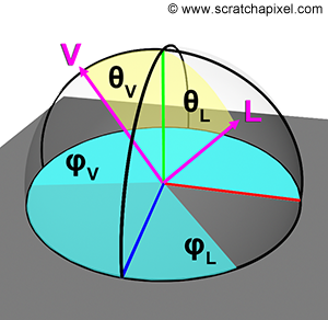
In the context of shading, as you may have guessed, the sphere and the hemisphere play an important role, and using spherical coordinates is going to be handy. For instance, BRDFs are functions of the incoming light direction (L) and outgoing viewing direction (V). Rather than using Cartesian coordinates to define these vectors, we can use spherical coordinates instead. Thus it reduces the BRDF from a function of six variables (two times three coordinates) to four variables only (two times two angles). To go from spherical coordinates to Cartesian coordinates, we can use the following equation (assuming the y-axis is the up vector. If you use a coordinate system in which the z-axis is the up vector, as often in shading, just swap the y and z coordinates in the following equations):

You can as easily go from Cartesian coordinates to spherical coordinates using the following formula (here again don't forget to swap the y and z coordinates if you use a coordinate system where the z-axis is the up vector):

More information on spherical coordinates can be found in the lesson on Geometry. Be careful though, note that in this less, we use the y-axis as the up vector, not the z-axis. These formulas can be implemented using the following C++ code. Keep in mind that if the vector is normalized its length is 1 thus \(r\) equals 1\. In that case, the division of z by r is not required of course. Also note that when x y and z are computed from the trigonometric function, the resulting vector is normalized. Finally, when the vector has normalized the value of the vector's y coordinates is the cosine of the angle \(\theta\):

// assuming all angles in radians
float theta = deg2rad(theta_deg); 
float phi = deg2rad(phi_deg);
float x = sin(theta) * cos(phi);
float y = cos(theta); 
// swap y and z if z-axis is up
float z = sin(theta) * sin(phi);
// r = 1 in this case because xyz is computed from trig functions
float r = sqrtf(x * x + y * y + z * z);
float theta = acos(y / r);
// use z if z-axis is up
float phi = atan2(z, x); 
// use y instead of z if z-axis is up
float costTeta = y;

We can also use a simple trick to compute theta from the Cartesian coordinates. Since \(r = \sqrt{x^2 + y^2 + z^2}\), we can write \(r^2 = x^2 + y^2 + z^2\). By arranging the terms we get \(y^2 = r^2 - x^2 - z^2\); y is the cosine of the angle theta, thus \(\cos(\theta) = \sqrt{r^2 - x^2 - z^2}\) and since \(r^2\) is equal to 1 when the vector is normalized, we finally get \(\cos(\theta) = \sqrt{1 - x^2 - z^2}\).

Differential and Integral Calculus

Besides trigonometry and geometry, two of the other most important tools used in the field of shading are integrals and differentials. These belong to a field of mathematics known as calculus: "calculus is the mathematical study of change, in the same way, that geometry is the study of shape and algebra is the study of operations and their application to solving equations". Both concepts are incredibly simple (and related to each other in a way we will explain now) when you know a few basic things about them.

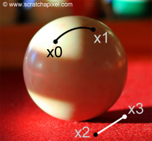
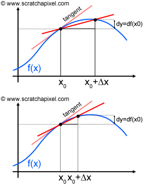
Let's start with differentials. In computer graphics, we often have to deal with functions. Measuring the amount of light arriving at a point on a surface can be seen as a function which we could write as \({Light_{incoming}} = f(x)\) where \(x\) here denotes a point on the surface. What this equation tells us is that the amount of light arriving on a point from the surface of an object is a function of this point's position in 3D space (Figure 3). Simpler examples can be found such as the position of a moving ball as a function of time which we can write as \(p = f(t)\). Many times we will want to know how this function changes within the proximity of \(x\) which we note \(f(x + \Delta x)\). In mathematical notation, the symbol \(\Delta x\) (the greek upper case letter delta) generally refers to a very small difference between two points (where these points are the input value of the function's argument). We have illustrated the concept in Figure 4\. If we plot the result of a function \(f(x)\) at two positions, \(x\) and \(x + \Delta x\) we can then trace a secant line between these two points. As \(\Delta x\) approaches zero, we can see (Figure 4) that the line passing through these two points gives a more precise approximation of the tangent line at \(x\). The tangent line is the limit of the secant line, as \(\Delta x\) approaches zero. The slope of this line is equal to the derivative of the function \(f\) at \(x\) and can be computed as \(dy\) (the difference between \(f(x + \Delta x)\) and \(f(x)\)) divided by \(\Delta x\):

The function difference divided by the point difference is known as the difference quotient. The value \(m\) which we know now is the slope of our function at \(x\) is also what is called the rate of change. Formally, the derivative of the function f at x is the limit of the difference quotient as \(\Delta x\) approaches zero:

If this limit exists, we then say that \(f\) is differentiable at \(x\). Several notations can be used to indicate a function's derivative. The most common (and modern) way is to add a prime mark to the function's name as in \(f'(x)\). This is known as Lagrange's notation. You can also use Leibniz's notation in which the derivative is noted as \({{d\over dx}f(x)}\) or \({{{df}\over dx}(x)}\) (the term \({d \over dx}\) is called the derivative operator and you should read it as "derivative with respect to x of the function f"). These are the most common notations used in computer graphics.

For quite a few functions, rules exist to find these functions' derivatives. For instance, the derivative of a constant is zero, and the derivative of any function of the type \(f(x) = x^n\) where \(n\) is any rational exponent is \(f'(x) = n x ^{n-1}\). This is known as the power rule and is very commonly used in computer graphics. However, finding the derivative of a function using an analytic solution is not always possible. Hopefully though in such cases, the limit of a function can generally be efficiently computed using numerical approximation instead. For instance, you can compute the function twice for values of \(x\) close to each other, and take the difference between the two results to obtain an approximation of the limit. In computer graphics, a lot of functions are discretized. Computing the differential of a discretized function at any \(x\) (assuming the function is one-dimensional), requires taking the difference between the sample at x and the value of the function at x + 1 (where x here is a discrete sample position). The resulting mathematical expression is called a finite difference. Note that if we divide the result of a finite difference by \(\Delta x\), we obtain a difference quotient. If we have a function \(f\), then \(F\) is the function \(f\) antiderivative if \(F' = f\). As a concrete example if you have the function \(x^2 + 1\) then the derivative of this function would be (using the power rule) \(2x\) (remember the derivative of a constant is zero since it doesn't change with respect to x). The antiderivative of \(2x\) is \(x^2\) however constants disappear when we take the derivative of a function, thus in the most generic case you should consider that the antiderivative of any function includes a constant. The correct answer (at least the most generic) is: \(x^2 + c\) where \(c\) denotes a constant. To summarize if:

• \(f\) is the derivative of \(F\) then,

• \(F\) is the antiderivative of \(f\)

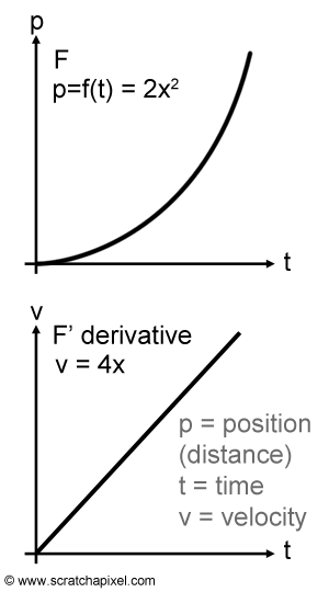
If we use the example of a function \(p = f(t)\) that gives us the position (or the distance) of a moving object with respect to time, then the derivative of this function \({dp \over dt}\) would give us velocity (change of position with respect to time) and the antiderivative of velocity would give us the position with respect to time (the original function \(p = f(t)\). Remember that velocity times time gives position. We illustrated this idea in Figure 6, where the graph at the top represents the position with respect to time function (\(F\)) and the bottom graph is a plot of this function's velocity (\(F'\) or \(f\)). We chose the function (\(2x^2\)) so that its derivative (velocity) can easily be computed using the power rule (\(4x\)). Note that since in this case, velocity (\(4x\)) is a linear function (a polynomial function of degree one), the plot is a straight line. Keep this example in mind as we will use it again for integrals.

Let's now have a look at integrals. Integrals and antiderivatives are actually the same thing. Because talking about the antiderivative of a function is not necessarily straightforward we will use some sort of notation instead. The antiderivative of the function \(2x\) we have been using before can be written using the following convention:

The expression above is called the indefinite integral of 2x which is another way of saying the antiderivative of 2x. You will understand why we use the term indefinite here in a moment. The most important thing to remember for now is that this big elongated S sign means an integral and that an integral is nothing else than the antiderivative of a function (remember that a derivative gives us the slope of the tangent line at any point).

If we get back to our example of a function \(F(t)\) giving us the distance of an object with respect to time, let's now imagine that we need to calculate the difference in position between time \(a\) and time \(b\) using velocity (which remember, is the derivative of \(F(t)\)). As an example, let's take \(a\) equals zero and \(b\) equal five seconds. In other words, we want to know how far has the object gone after five seconds. Obviously, computing this value using \(F(t)\), the antiderivative is easy; we just need to write:

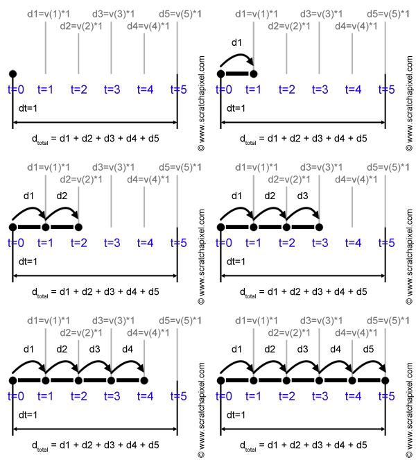
But let's assume here that we only have velocity (the derivative) to work out the distance traveled by the object over five seconds. Since velocity times time gives a distance, we can assume that if we take the velocity at time \(t = 1\), the distance the object has traveled at that time is the velocity at time \(t =1 \) times one (velocity times time). We then want to compute the distance the object has traveled from time \(t=1\) to time \(t = 2\). This distance can be evaluated again by multiplying the velocity of the object at time \(t=2\) by one, which is the time it took for the object to travel from \(t=1\) to \(t= 2\). In mathematical notation, we generally refer to this time step as \(dt\). If we repeat this process for the remaining three seconds (until we reach \(t = 5\)), then for each time fragment, we have a value indicating the distance traveled by the object from time \(t\) to time \(t + dt\). Summing up the distances traveled by the object during each one of these five-time steps gives us an "approximation" (we will explain why in a moment) of the overall distance traveled by the object from time \(t=0\) to time \(t = 5\) (see Figure 7). If we apply this method using the derivative of \(2x^2\), which is \(4x\), we get:

As you can see the values we computed using the antiderivative \(^2\) and the value we computed using the derivative \(4x\) are different. We mentioned before that the method using the derivative gives an approximation and we will soon explain why. We will also show how the error can be reduced.

Let's summarize what we have learned so far. We learned that to compute the change \(X\) of a certain antiderivative \(F(x)\) over a given interval defined by the upper and lower limits \(a\) and \(b\), we can use the following equation:

We have also learned how to calculate an approximation of \(X\) using \(f(x)\), \(F(x)\)'s derivative. To do so, we need to evaluate \(f(x)\) at regular intervals \(dx\) between \(a\) and \(b\) multiply these values by \(dx\) and then add up the results:

This sum can be written in a more compact form using the following mathematical convention:

Where the symbol \(\sum\) means "sum" (the upper case greek letter sigma). In mathematics, this formulation is known as a Riemann sum (named after German mathematician Bernhard Riemann). Note that in the Riemann sum:

where N again is the number of subintervals used in calculating an approximation of \(X\). In a Riemann sum, \(dx\) is usually regular but it doesn't have to be.

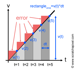
Let's now imagine that we have a velocity function similar to the one we represented in Figure 6 (bottom). On this graph, since we have computed the distance traveled by the object over a time step \(dt\) as \(v(t)\) times \(dt\), we can represent this distance on the graph as a small rectangle (also sometimes called a partition) where the width and length of this rectangle are \(dt\) and \(v(t)\) respectively (Figure 8). Since to calculate an approximation of the overall distance traveled by the object from t=0 to t=5 we added up the distances traveled by the object over short regular time step \(dt\) taken a regular interval from t=0 to t=5, and since we can represent each one of these distances as rectangles on the graph, the overall distance we have calculated can also be seen as the sum of these rectangles' area where the area of the rectangle here is calculated as \(v(t)\) times \(dt\). The equation we used before:

can thus be seen as a sum of the rectangles' area under the velocity curve. And the sum of these rectangle's area can also be seen as an "approximation" of the area below the curve from \(a\) to \(b\). You can also see why this sum of rectangles' area only represents an approximation of the real area under the curve. In Figure 9 we have highlighted in red, the part of the rectangles which is above the curve to better show how they overestimate the real area under the fragment of the curve they overlap. This explains why the approximation we found for d using the derivative method (60) is greater than the exact value calculated using the antiderivative method (50). We also said before that we would show how to reduce this error. If you haven't found yet how this can be achieved, try to imagine what happens if we take smaller \(dt\) steps. We end up increasing the number of rectangles used in the approximation of the area under the curve but as you can hopefully see in Figure 10, the part of the rectangle lying outside the limit of the curve is also reduced (the difference in the error between the approximation used in Figure 9 and Figure 10 is highlighted in red in Figure 10), thus we get a more precise approximation (but it stays an approximation, only a better one). If we can keep reducing \(dx\) then of course the error keeps getting smaller and smaller. The question is now what happens to this approximation as \(dx\) approaches zero? If you haven't guess yet, the number of rectangles becomes infinitely big as \(dx\) approaches zero and we end up (in theory) with the exact value for the area under the curve between point \(a\) and point \(b\). And this is in essence exactly what an integral is. In other words:

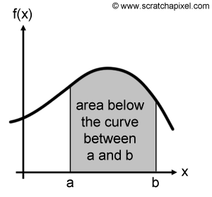
The sum of the rectangles area below the curve as \(dx\) approaches zero, is equal to the definite integral (definite in this case because the integral is computed between \(a\) and \(b\)) of a function f(x) which is also similar to the area below the curve defined by the function between point \(a\) and point \(b\) (Figure 11). In other words, you can see an integral as being nothing else really than a sum: the sum of the height at any given point between \(a\) and \(b\) times the base of the rectangle which is \(dx\). This what a definite integral is. In a computer program we usually give \(dx\) a small value and as mentioned before the smaller the value the smaller the error (but the longer it takes to compute the integral). Here for example a C++ program which you can use to compute the change of distance between two given point in time using both the antiderivative function (\(2x^2\)) and the derivative function (\(4x\)) using the integral method:

#include <cstdlib> 
#include <cstdio> 
 
float F(float x) { return 2 * x * x; } 
float f(float x) { return 4 * x; } 
 
int main(int argc, char **argv) 
{ 
	float a = atof(argv[1]); 
	float b = atof(argv[2]); 
	int N = atoi(argv[3]); 
	float exact = F(b) - F(a); 
 
	// compute approximation using Riemann sum 
	float dt = (b - a) / N, time = dt, sum = 0; 
	for (int i = 1; i <= N; ++i) { 
		float delta_d = f(time) * dt; 
		sum += delta_d; 
		time += dt; 
	} 
	printf("Result, exact %f, approximation %f, diff %f\n", exact, sum, sum - exact); 
 
	return 0; 
} 

You can compile this program will the following command and run it like this:

c++ -o derivative derivative.cpp -O3 
./derivative 0 5 100 

where the first two arguments are the boundaries of the integral (the interval of integration [a,b]) and the third argument the number of rectangles in the Riemann sum we wish to use to evaluate this integral. If you run this program several times, you will see that the error decreases and the number of partitions increases. In mathematical form, the value for the arguments to the program we used in this example would correspond to the following equations:

with:

This is what the program above calculates. One of the most important things to remember with integrals is that we have been able to compute the result of the integral with the integral's function antiderivative. Remember than we computed the change of a certain antiderivative \(F(x)\) in the interval \([a,b]\) using the following equation: \(X = F(b) - F(a)\). We compute the same value using the function derivative using the integral formulation: \(\int_a^b f(x)dx\) thus we can write the following equality:

Where f(x) is the derivative of F(x) and F(x) is the antiderivative of f(x). This is an extremely important relation which is known in calculus as the second fundamental theorem of calculus. Where, in mathematics, the expression \(F(b) - F(a)\) is usually defined using the following notation:

As an example, imagine that you want to calculate the integral of \(4x\) in the interval \([0,5]\) using the second fundamental theorem of calculus. This approach is usually only possible if you can easily find the antiderivative of the integral's function. In this simple case, we know that antiderivative of \(4x\) is \(2x^2\) thus we can write:

This technique is often used in computer graphics because especially when it comes to shading, we constantly need to compute integrals, particularly integrals involving trigonometric functions. These derivatives (and their inverses) can easily be found on the web, thus we won't include them here. As an example (we will be using the integral of the cosine function in the next chapters), imagine you want to integrate the cosine function over the interval \([0:\pi]\):

The antiderivative of the cosine function is the sine function, thus using the second fundamental theorem of calculus we can write:

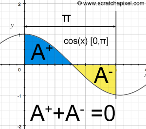
This result is expected because if you graph the cosine function in the range \([0,\pi]\) and look at the integral as the signed area below the curve in this given interval, then as you can in Figure 12, this area is zero (the "positive" area in the interval \([0,\pi/2]\) is cancelled out by the "negative" area in the interval \([\pi/2:\pi]\)).

So far we have only worked with function defined in one dimension (\(f(x)\) takes one variable only, \(x\)), but differentiation and integration can also be applied to two and three dimensional functions. For example in the two-dimensional case, we may want to integrate the function \(x = f(x, y)\) where \(x\) and \(y\) are the two variables of the function. When graphed, such a function would give a surface (Figure 13). Let's now write the integral of this function:

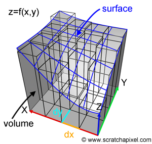
Similarly to the one-dimensional case, we need to bound the surface to some intervals both along the x-axis as well as along the y-axis, defining what we call the domain of integration (the range of values in x and y over which the integration is performed). And similarly to the one-dimensional case, we will "divide" the surface into small partitions but since we deal with a surface rather than a curve, these partitions are defined in the xy plane and have dimension \(dx\) and \(dy\) respectively. The function \(f(z,y)\) returns a height \(z\) which multiplied by \(dx\) and \(dy\) gives the area of an elongated cube under the surface. When the area of all these cubes is added up, we get an approximation of the volume under the surface (as shown in Figure 13). The Riemann sum in the one and two-dimensional case works the same.

In conclusion, the integral of a one-dimension function \(f(x)\) can be seen as the area under the curve, while the integral of a two-dimensional function \(f(x,y)\) can be interpreted as the volume under the surface. Let's comment on looking at the three-dimensional case.

We repeated many times now that the integral of a one-dimensional function in a given interval (the domain of integration), is "similar" to the area under the curve in this interval. The problem with saying that calculating an integral is the same as calculating the area under the curve is to avoid seeing this interpretation as the only and literal possible interpretation of an integral. In reality, you should always consider the context of the problem in which the integral is used to interpret what the meaning of the integral may be. For instance, in one of the lessons on shading, we show that ray tracing is a means by which we can compute a radiometric quantity called radiance over the area of a pixel. In this particular example because we deal with a two-dimensional function (radiance as a function of the position of a point on the surface of a pixel) we can express this problem as a double integral (one over x and one over y). The result of this integral is not as literally speaking the "volume" under the function (where here the function is the radiance quantity we want to measure) but is more accurately defined in this context, as the radiance area density (in another world as radiance per square units where unit here denotes a distance measured in meters, centimeters, feet, inches, etc.). Imagine that you need to measure the density of leaves on a flat surface (e.i. the number of leaves per square meter). Assuming the distribution of leaves is not uniform, to measure the density of leaves at any local position on this surface, you will need to define an area (the domain of integration) and divide this area into equally spaced partitions (\(dx\) and \(dy\)). Let's say that the width of each one of these partitions is one (thus the area of a partition is one square meter). Then if you count the number of leaves contained in any given partition, you effectively have a measure of the leaf area density for this partition (Figure 14). But you could also write this measure, as an integral over the area of the partition:

The function \(f(x)\) would return the number of leaves at any given point \(x\) in a partition \(P\) of area \(A\) within a small surface element \(dA\) around \(x\) (e.i. leaves per square meters for instance).

Now that we suggested that an integral could also be looked at as representing an area density, the task of understanding three-dimensional integrals should be easier. Similarly to the case of having to calculate the volume of water contained in a tank while only using a function returning the height of any point on the water surface as a function of a position in the 2D plane, imagine that you now want to calculate the density (e.i the mass per unit volume) of a non-homogeneous material. By heterogeneous we mean that density varies between different regions of the object. Note that density itself could be defined as a function of a point in 3D space such as \(\rho = f(x,y,z)\) (density is usually denoted with the greek letter rho, \(\rho\)). The domain of integration is the region in which we want to measure the density of the object (the cube in figure 15). The density is assumed to vary across space, however, we can assume that within a very small region of this object, the density is homogeneous. Thus similarly to the technique used with curves and surfaces, we will integrate the density function over the domain of integration using the Riemann sum approach, where the volume of the object for which we need to calculate density will be divided into small 3D partitions with extent \(dx\), \(dy\) and \(dz\). The density is evaluated at these positions, multiplied by the volume of the partition (\(dx * dy * dz\)) and the results are summed up:

In figure 15, N=M=0=10\. As usual, as \(dx\), \(dy\), and \(dz\) approach zero, we can write the Riemann sum as a triple integral:

Again, the integral in the case is better interpreted as an indication of the area density of the function we integrate. In our example, the density of an object within a volume is defined by some intervals in each dimension (our domain of integration).

Integrals are not limited to three dimensions. We can have as many dimensions as we want, and we will soon see that in fact, many equations in rendering involve multi-dimensional integrals with more than three dimensions (where these dimensions don't have to be positioned in space or directions, but can also be time for instance). We will present these equations in the lessons of volume 2 (Rendering Equation).

Conclusion: the Mathematics of Rendering Demystified

The mathematical tools presented in this chapter are used in almost every algorithm related to rendering, particularly integration. In this chapter, we hopefully explained what they are, and how and why they work simply and intuitively. You can hardly (really) understand the theory and practical implementation of computer graphics algorithms if you do not know what differentiation and integration are, however, if you made the effort to read this lesson, you now understand these techniques better and will hopefully agree that there's nothing difficult about them.