Monte Carlo in Rendering (A Practical Example)
Reading time: 13 mins.Rendering the McBeth Chart using Monte Carlo Integration

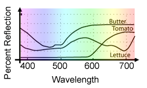
In the lesson on Colors and Digital Images, we explained that colors could be represented as curves giving the amount of light at each wavelength (denoted with the greek letter lambda \(\lambda\)) in the visible spectrum (these curves are called spectral power distribution or SPD). Examples of such curves for three different materials are shown in Figure 1. As you can see, these curves can be interpreted as a function of wavelength: f(\(\lambda\)). Generally, the visible spectrum is considered to be within the interval of 380 to 730 nanometers. To convert this curve back to tristimulus values X, Y, and Z, we need to calculate three one-dimensional integrals:
$$ \begin{array}{l}X = \int_{\lambda1}^{\lambda2} spd(\lambda) \bar X(\lambda) d\lambda\\Y = \int_{\lambda1}^{\lambda2} spd(\lambda) \bar Y(\lambda) d\lambda\\Z = \int_{\lambda1}^{\lambda2} spd(\lambda) \bar Z(\lambda) d\lambda \end{array}. $$Where the functions \(\bar X, \bar Y, \bar Z\) are the CIE standard observer color matching functions. The resulting tristimulus values X, Y, and Z can then be converted to RGB. We explained this process in detail in the lesson on Color and Digital Images.
Hopefully, you have guessed that we were going to use Monte Carlo integration to solve these integrals. The SPDs we will be using is the spectral data for each of the 24 different colors used on a McBeth chart. Spectral data for these colors are readily available on the web. If you remember what we said about Monte Carlo integration in the previous chapter, this estimator is defined as:
$$\langle F^N \rangle = (b-a) \dfrac{1}{N} \sum_{i=0}^{N-1} f(X_i).$$In our example, the interval [a,b] is [380,730] the range of wavelength defining the visible spectrum. To approximate the XYX values for each color of this color checker, we need to choose a random wavelength within this interval, evaluate and multiply with each other the spd and the color matching functions at this random wavelength, repeat this process N times (where N is the number of samples), sum up all the results, divide the final number by N, and multiply it by (b-a). In pseudo-code we get:
int N = 32;
float lambdaMin = 380, lambdaMax = 730;
float X = 0, Y = 0, Z = 0;
for (int i = 0; i < N; ++i) { // for each sample
    // select a random wavelength
    float lambda = lambdaMin + drand48() * (lambdaMax - lambdaMin);
    // evaluate the sod and the color-matching function at this wavelength,
    // multiply the results, and add the contribution of these samples to the others
    X += spd(lambda) * CIE_X(lambda);
    Y += spd(lambda) * CIE_Y(lambda);
    Z += spd(lambda) * CIE_Z(lambda);
}
// complete the integral, multiply by (b-a) and divide by N
X *= (lambdaMax - lambdaMin) / N;
Y *= (lambdaMax - lambdaMin) / N;
Z *= (lambdaMax - lambdaMin) / N;

Simple? Indeed. To illustrate what variance is, we will render each color of the MacBeth chart as a 64x64 square using MC integration for each pixel of that square (each pixel of a color bucket, is obtained by running a new Monte Carlo simulation and therefore each pixel is likely to be "slightly" different than the others. How different depends mostly on the number of samples N used in the simulation). Our final goal is to recreate something that looks like a real McBeth chart, but CG generated (and using Monte Carlo integration of course). In lesson 5, we provided the source code of a small program rendering a McBeth chart using a Riemann sum to compute the integrals. We will start from this program as it already contains the spectral data for the McBeth chart as well as the CIE color-matching functions. The heart of the code is the function in which the Monte Carlo integration is done.
unsigned int N = 32;

inline float linerp(const float *f, const short &i, const float &t, const int &max)
{ return f[i] * (1 - t) + f[std::min(max, i + 1)] * t; }

void monteCarloIntegration(const short &curveIndex, float &X, float &Y, float &Z)
{
    float S = 0; // sum, used to normalize XYZ values
    for (int i = 0; i < N; ++i) {
        float lambda = drand48() * (lambdaMax - lambdaMin);
        float b = lambda / 10;
        short j = (short)b;
        float t = b - j;
        // interpolate
        float fx = linerp(spd[curveIndex], j, t, nbins - 1);
        b = lambda / 5;
        j = (short)b;
        t = b - j;
        X += linerp(CIE_X, j, t, 2 * nbins - 1) * fx;
        Y += linerp(CIE_Y, j, t, 2 * nbins - 1) * fx;
        Z += linerp(CIE_Z, j, t, 2 * nbins - 1) * fx;
        S += linerp(CIE_Y, j, t, 2 * nbins - 1);
    }
    // sum, normalization factor
    S *= (lambdaMax - lambdaMin) / N;
    // integral = (b-a) * 1/N * sum_{i=0}^{N-1} f(X_i) and normalize
    X *= (lambdaMax - lambdaMin) / N / S;
    Y *= (lambdaMax - lambdaMin) / N / S;
    Z *= (lambdaMax - lambdaMin) / N / S;
}
As you can see with this code, we first sample a random value for the wavelength contained in the interval [380,730] (line 10). we need to convert this random wavelength to an index for performing a lookup into the CIE color matching functions (sampled every 5 nm) and McBeth spectral data (sampled every 10 nm) 1-D tables. Because the wavelength may fall between two samples in the table, it is best to perform a linear interpolation (interpolate the two nearest samples). Finally, X, Y, and Z are updated with the value of the CIE color-matching function and spectral data at this wavelength (lines 19-21). Because these values will need to be normalized (check lesson 5), we also need to compute the integral of the CIE color-matching function corresponding to the Y component. Here as well, we can use a Monte Carlo integration (line 22). Finally, the X, Y, and Z values are multiplied by (b-a) (in this example the minimum and maximum wavelength) and divided by N (lines 27-29). We also have to normalize them but this has nothing to do with an MC integration (it is just part of the process of converting spectral data to XYZ).
const double XYZ_to_RGB[][3] = {
    { 2.3706743, -0.9000405, -0.4706338},
    {-0.5138850,  1.4253036,  0.0885814},
    { 0.0052982, -0.0146949,  1.0093968}
};

void XYZtoRGB(const float &X, const float &Y, const float &Z, float &r, float &g, float &b)
{
    r = std::max(0., X * XYZ_to_RGB[0][0] + Y * XYZ_to_RGB[0][1] + Z * XYZ_to_RGB[0][2]);
    g = std::max(0., X * XYZ_to_RGB[1][0] + Y * XYZ_to_RGB[1][1] + Z * XYZ_to_RGB[1][2]);
    b = std::max(0., X * XYZ_to_RGB[2][0] + Y * XYZ_to_RGB[2][1] + Z * XYZ_to_RGB[2][2]);
}

int main(int argc, char **argv)
{
    ...
    for (int y = 0, pixIndex = 0; y < height; ++y) {
        short row = (short)(y / squareSize);
        for (int x = 0; x < width; ++x, pixIndex++) {
            short column = (short)(x / squareSize);
            // compute each pixel of the square
            float X = 0, Y = 0, Z = 0;
            monteCarloIntegration(row * 6 + column, X, Y, Z);
            float r, g, b;
            XYZtoRGB(X, Y, Z, r, g, b);
            buffer[pixIndex][0] += r;
            buffer[pixIndex][1] += g;
            buffer[pixIndex][2] += b;
        }
    }
    ...
}

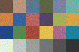
The main function of the program loops over each pixel of the frame. For each pixel, it computes the row and column this pixel corresponds to in the McBeth chart (the squares of the chart are organized as a series of 4 rows and 6 columns. You can see an example of the McBeth chart in figure 2). The spectral data of that color will be used to compute a value for X, Y, and Z (lines 22 and 23). Then they are converted to RGB values, a process which we also explained in the lesson Introduction to Light, Color, and Color Space. Finally, these RGB values are stored in a buffer which is then save to disk once all the pixels are processed (your screen is likely to expect your image to be in sRGB so we also apply gamma to the pixel values before storing them to disk). The result for 32 samples can be seen in Figure 3. Now as you can see the result is far from being bad, but the image is quite noisy! This is the famous variance, we have been talking about in the lesson Mathematical Foundations of Monte Carlo Methods. Or what you call maybe more commonly noise when you look at your renders.
Example of Progressive Rendering
To demonstrate another very nice property of Monte Carlo integration, we will modify our program so that it keeps refining the result by computing as many version of this image as we want (we will call these images passes) and averaging their results. In a way, it is the same as increasing the number of samples N. However if had increased N to 4096 for instance, the image might have taken a much longer time to render (in fact, technically 128 times longer than an image for which N = 32). Thus when N is small, we can see a result right away, and if we like what we see after this quick first pass, then we can let the program run and compute more passes until we are eventually satisfied with the image quality (that is when you think the noise is not distracting anymore). This method is known as progressive rendering. Imagine you need to deliver a sequence of images by a certain time. If X is the number of minutes you get when you divide the total number of rendering time you have by the total number of images you need to render, then you can let your program render each one of these images for no longer than X minutes. That way, you are certain that all your images will be rendered on time. They might have some noise, but you will have a complete sequence of images to look at, and, in some circumstances, this is often better than having an incomplete sequence of images even if they look much better. The fact that render time is predictable, is generally useful in a production environment. Also, if you like the sequence of images that you get after X hours of render time, you can re-launch the sequence and let it refine for another X number of hours. Rather than rendering each image from scratch again, the program can simply start from the existing renders and keep refining them by adding more passes. Therefore, no rendering resources are wasted! These are some of the great benefits of progressive rendering.
More formally, remember that a Monte Carlo integration is just like computing the sample mean of a random variable. In the lesson Mathematical Foundations of Monte Carlo Methods, we explained in detail that these samples' means (which are themselves random numbers) can also be averaged to produce more accurate results. In this example, a pass is nothing else than a sample mean. And the result of these passes can be averaged to produce a more accurate result (as with sample means). This is why Monte Carlo integration makes progressive rendering possible.
We have implemented a basic form of progressive rendering in our program. This time we won't display the result in an OpenGL window. The program runs entirely in a shell. It will keep rendering passes and accumulating the results in the buffer until the user terminates the program (using ctrl-c). The program will catch this signal and will call a function in which we will save the result of the buffer to disk before quitting. Note that in fact, after each passe, we will actually convert the content of the buffer to a proper image in which the content of the buffer is divided by the total number of passes (the buffer is like an accumulation buffer). It is the content of the image which is saved to disk, not the buffer. Here is the source code:
void handler(int s)
{
    printf("Saving image after %d passes\n", npasses);
    std::ofstream ofs;
    ofs.open("./mcbeth.ppm");
    ofs << "P6\n" << width << " " << height << "\n255\n";
    for (uint32_t i = 0; i < width * height; ++i) {
        unsigned char r, g, b;
        r = (unsigned char)(std::min(1.f, pixels[i][0]) * 255);
        g = (unsigned char)(std::min(1.f, pixels[i][1]) * 255);
        b = (unsigned char)(std::min(1.f, pixels[i][2]) * 255);
        ofs << r << g << b;
    }
    ofs.close();
    exit(0);
}

int main(int argc, char **argv)
{
    pixels = new color[width * height];
    memset(pixels, 0x0, sizeof(color) * width * height);
    buffer = new color [width * height];
    memset(buffer, 0x0, sizeof(color) * width * height);
    struct sigaction sigIntHandler;
    sigIntHandler.sa_handler = handler;
    sigemptyset(&sigIntHandler.sa_mask);
    sigIntHandler.sa_flags = 0;
    sigaction(SIGINT, &sigIntHandler, NULL);
    static const float gamma = 1 / 2.2;
    while (1) {
        for (int y = 0, pixIndex = 0; y < height; ++y) {
            short row = (short)(y / squareSize);
            for (int x = 0; x < width; ++x, pixIndex++) {
                short column = (short)(x / squareSize);
                // compute each pixel of the square
                float X = 0, Y = 0, Z = 0;
                monteCarloIntegration(row * 6 + column, X, Y, Z);
                float r, g, b;
                XYZtoRGB(X, Y, Z, r, g, b);
                buffer[pixIndex][0] += r;
                buffer[pixIndex][1] += g;
                buffer[pixIndex][2] += b;
            }
        }
        npasses++;
        for (uint32_t i = 0; i < width * height; ++i) {
            pixels[i][0] = powf(buffer[i][0] / npasses, gamma);
            pixels[i][1] = powf(buffer[i][1] / npasses, gamma);
            pixels[i][2] = powf(buffer[i][2] / npasses, gamma);
        }
        printf("npasses %3d (num samples %5d)\n", npasses, npasses * N);
    }
    delete [] pixels;
    delete [] buffer;
    return 0;
}
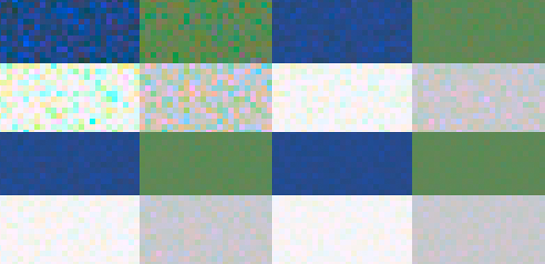
Let's look at some results. The following sequence of images shows the result after 1, 8, 16, and 32 passes (this corresponds to 32, 256, 512, and 1024 samples respectively).

Obviously, as expected the noise is reduced as the number of passes (i.e. the number of samples) increases. By zooming out on a section of these images, we can see the noise better. Keep in mind that in Monte Carlo, you need 4 times as many samples to reduce the noise (or variance) by 2.

As suggested already a couple of times throughout this lesson, the art of Monte Carlo rendering is mostly about finding ways of reducing this noise. We will talk about variance-reduction techniques later in this lesson.
Conclusion
Hopefully, with this exercise, you better understand what Monte Carlo integration is, which as you can see is not only a simple idea but also really straightforward to implement. You also have a simple program that demonstrates the concept of progressive rendering (which is only possible because of the nature of the Monte Carlo algorithm). You hopefully now have a better understanding of where the noise (or variance if you use the correct technical term) comes from in your renders. And if you see this noise in our 3D renders, you can be sure that the renderer that produced this image, uses some sort of Monte Carlo integration.
Exercice
Adapt the program to display the image each time a new pass is added in an OpenGL window.
Adapt the program to stop the render after a given time.