Value Noise and Procedural Patterns

Creating a Simple 1D Noise

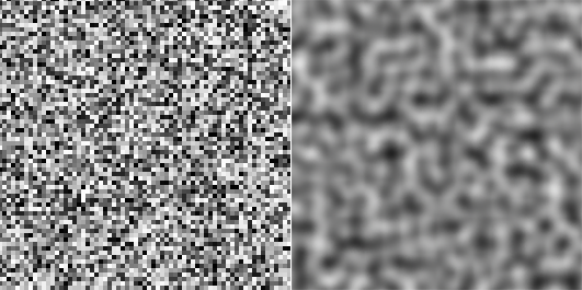
Noise is a function that returns a float in the range [0:1] for a specific input x (x can be a float, a 2D, 3D, or 4D point, but in this chapter, we will only be looking at the one-dimensional case. Our input position can also be positive and negative and extend from 0 to infinity or minus infinity). We could generate these floats using a random number generator but we have explained in the first chapter that it returns values that are very different from each other each time the function is called. This creates a pattern known as white noise which is not suitable for texture generation (white noise patterns are not smooth while most natural patterns in nature are).

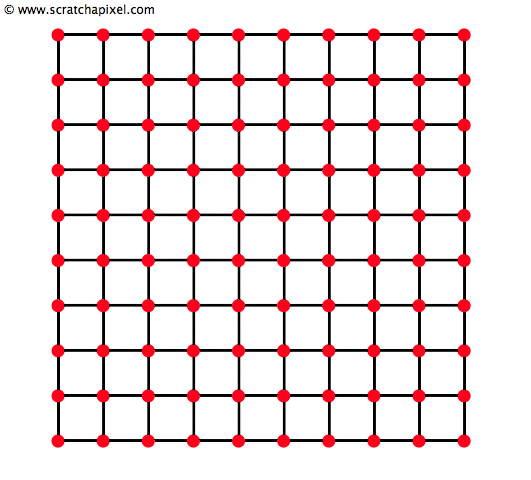
Instead, we will create a series of random points (using drand48()) spaced at regular intervals. If you work in 2D, we create these random values on the vertices of a regular grid (lattice); if you work in 1D, this grid can be seen as a ruler. To make things simple, we will assume that the vertices of that grid or the ticks on that ruler are created at coordinates along the x and y axis, which have integer values (0, 1, 2, 3, etc.). These random numbers are generated at these positions only once (when the noise function is initialized).

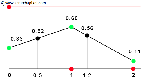
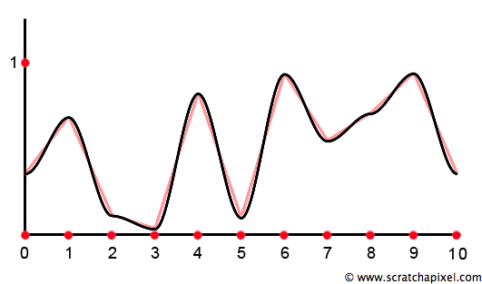
If we continue with our 1D example, we can see that we are left with a series of dots or values defined at the integer position on the ruler. For example, the result of the function for x = 0 is 0.36, the result for x = 1 is 0.68, etc. But what results from that function when x is not an integer? To compute a value for any point on the x-axis, we need to find out the two nearest integer positions on the x-axis for this input value (the minimum and the maximum) and use the random values that are associated with these two positions. For instance, if x equals 0.5, the two points with integer values surrounding x are 0 and 1. And these two points have the associated random values 0.36 and 0.68. The result of the function for x, when x = 0.5, is a mix of the value 0.36 defined at point 1 and the value 0.68 defined at point 2. We can use a simple interpolation technique called linear interpolationto compute this number. Linear interpolation is a simple function that returns a mix of the values \(a\) and \(b\) for a specific value \(t\), where t is in the range [0:1]:

In the case of our noise function, we will replace \(a\) and \(b\) with the random values defined at the integer positions surrounding x (if x = 1.2, the random values for x = 1 and x = 2), and we will compute \(t\) from x, by simply subtracting the minimum integer value found for x from x itself (t = 1.2 - 1 = 0.2).

int xMin = (int)x; 
float t = x - xMin; 

And here is the code to compute a value using linear interpolation. In most shading language, this function is called lerp (for linear interpolation, of course):

template<typename T = float> 
inline T lerp(const T &lo, const T &hi, const T &t) 
{ return lo * (1 - t) + hi * t; } 

Computing a value for any x in the range [0:1] using linear interpolation is similar to drawing a line from point 1 to point 2. If we repeat this process for all the points in the range [1:2], [2:3], and so on, we get the curve from Figure 4. You may now understand why we call this type of noise value noise (noise can be created in a few different ways). The idea is to generate some values at regular intervals on a ruler (1D) or a grid (2D) and then use linear interpolation.

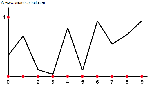
We now have all the bits and pieces we need to create a simple noise function. When initializing the function, we will create a series of random values, which we will store in a float array (the numbers written in boxes at the bottom of Figure 4). As you can see in the code, the array's length can easily be changed. This will be important later, but to keep the demonstration simple, we will only create 10 values (from the origin 0 to 9). The index of a number in the array corresponds to its position on the ruler. The first number in the array corresponds to x = 0, the second to x = 1, etc. To compute a noise value for x, we will first calculate the integer boundaries for x (the minimum and the maximum integer value for x). We can then use these two integer values as index positions in the array storing the random numbers. The two numbers we get, \(a\) and \(b\), are the two random values stored at these index positions. We also need to find \(t\) from x using the technique described above (subtract the minimum integer for x from x). The final step is to perform a linear interpolation of \(a\) and \(b\) using \(t\) by calling the mix function. And you get the result of the noise function for x.

class ValueNoise1D 
{ 
public: 
    ValueNoise1D( unsigned seed = 2011 ) 
    { 
        srand48(seed); 
        for (unsigned i = 0; i < kMaxVertices; ++i) { 
            r[i] = drand48(); 
        } 
    } 
 
    // Evaluate the noise function at position x
    float eval(const float &x) 
    { 
        int xMin = (int)x; 
        assert(xMin <= kMaxVertices - 1); 
        float t = x - xMin; 
 
        return lerp(r[xMin], r[xMin + 1], t); 
    } 
 
    static const unsigned kMaxVertices = 10; 
    float r[kMaxVertices]; 
}; 
 
int main(int argc, char **argv) 
{ 
    ValueNoise1D valueNoise1D; 
 
    static const int numSteps = 200; 
 
    for (int i = 0; i < numSteps; ++i) { 
        float x = i / float(numSteps - 1) * 10; 
        std::cout << "Noise at " << x << ": " << valueNoise1D.eval(x) << std::endl; 
    } 
 
    return 0; 
}

We only have 10 random values defined at each integer position on the x-axis starting at x = 0, so we can only compute a value for any x in the range [0:10]. Why [0:10] instead of [0:9]? When x is in the range [9:10], we will compute the random value at index 9 and 0 to compute a noise value. As you can see in figure 6, if you do this, the curve's beginning and end are the same. In other words, noise when x = 0 and when x = 10 is the same (in our example, 0.36). Let's copy the curve and move it to the left or the right of the existing one. The existing curve (curve 1) is defined over the range [0:10], and the new copy (curve 2) is defined over the range [10:20].

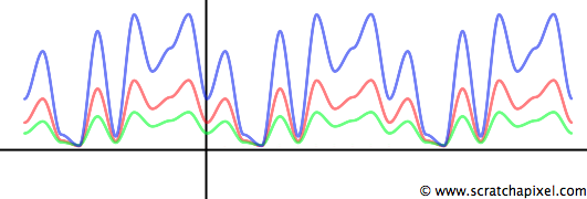
You can see that there are no discontinuities where the curves join (for x = 10). Why? Because the noise value at the end of curve 1 is the same as the noise value at the start of curve 2. And that's because when x is in the range [9:10], we interpolate the random value for x = 9 and x = 0. Because there are no discontinuities between successful copies of the curve, we can make as many copies as we want and extend our noise function to infinity. The value for x is not limited anymore to the range [0:10]. It can take any positive or negative values going from 0 to infinity (or minus infinity. The noise function should work for negative values as well).

How do we make that possible in the code? We know how to compute a noise value when x is in the range [0:9]. However, when x is greater than 9 (and the same thing applies for the case where x is negative), let's say 9.35, we want to interpolate the random position at x = 9 and x = 0, as explained above. If we take the minimum and maximum integer for x, we get 9 and 10. But instead of using 10, we want to use 0. What we need here is the modulo operator. The modulo operator gives the remainder of a number divided by another number (in our case, the remainder of x divided by 10). If you do the math, the remainder of 9 divided by 10 is 9. And the rest of 10 divided by 10 is 0. In other words, using the modulo operator on the minimum and maximum integer value for x = 9.35 gives us 9 and 0, which is precisely what we want. And if you do the test, you will see that using this operator always returns the proper integer boundaries for any x greater than 10 or lower than 0 (special care must be taken for negative values, but the principle is the same).

Using this technique, we can repeatedly cycle over the noise functions as we move along the x-axis (similar to making copies of the original curve). We mentioned in the first section that the noise function was periodic. In this case, the period of the function is 10 (it repeats itself every 10 units on each side of the origin for negative and positive values of x). We will now use the modulo operator (% in C++). Still, later on, we will see how this can be simplified and made more efficient (be aware that the following code does not work for values of x lower than 0. This restriction will be removed in the last version of this code snippet):

class ValueNoise1D 
{ 
public: 
    ValueNoise1D(unsigned seed = 2011) 
    { 
        srand48(seed); 
        for (unsigned i = 0; i < kMaxVertices; ++i) { 
            r[i] = drand48(); 
        } 
    } 
 
    // Evaluate the noise function at position x
    float eval(const float &x) 
    { 
        int xi = (int)x; 
        int xMin = xi % (int)kMaxVertices; 
        float t = x - xi; 
        int xMax = (xMin == kMaxVertices - 1) ? 0 : xMin + 1; 
 
        return lerp(r[xMin], r[xMax], t); 
    } 
    static const unsigned kMaxVertices = 10; 
    float r[kMaxVertices]; 
}; 
 
int main(int argc, char **argv) 
{ 
    ValueNoise1D valueNoise1D; 
 
    static const int numSteps = 200; 
 
    for (int i = 0; i < numSteps; ++i) { 
        float x = i / float(numSteps - 1) * 10; 
        std::cout << "Noise at " << x << ": " << valueNoise1D.eval( x ) << std::endl; 
    } 
 
    return 0; 
}

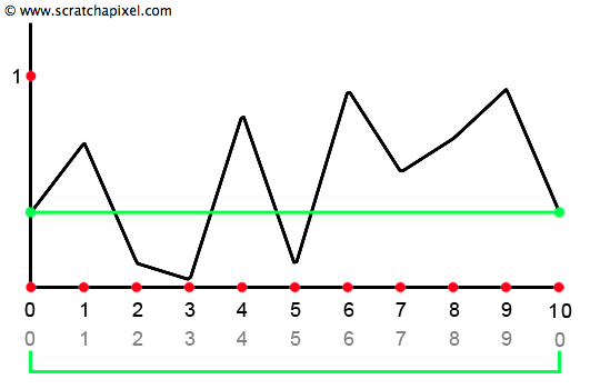
There is nothing wrong with this result (technically, it does the right thing) except that it looks like a saw-toothed curve which is not very natural. If you look at random patterns in nature, such as the profile of an ocean surface (waves), they usually do not have this saw-toothed profile. Their profile is smooth (rounded). What we can do to change the appearance of this curve is to remap our input \(t\) value using another function that has a smooth profile (a function that produces a curve having an "S" shape). Two S curve functions commonly used to remap t are the cosine and the smoothstep function. It is essential to understand that the code for interpolating the random values does not change. We remap the value of \(t\) before we use it in the mix function. Once again, we do not replace the mix function with an "S" curve function. We remap \(t\) using a smooth function followed by a linear interpolation of \(a\) and \(b\) using this remapped value of \(t\). Here is what we get in pseudo-code:

float smoothNoise(const float &a, const float &b, const float &t) 
{ 
    assert(t >= 0 && t <= 1);      //t should be in the range [0:1] 
    float tRemap = smoothFunc(t);  //remap t input value 
    return lerp(a, b, tRemap);     //return interpolation of a-b using new t 
} 

Cosine

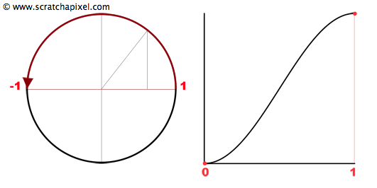
Let's start to plot the cosine function in the range [0:2Pi] (a complete turn around the unit circle). You are undoubtedly familiar with the profile of this curve (figure 7, left image). As you can see, the curve goes from 1 to 0 when x is in the range [0:Pi/2], 0 to -1 when x is in the range [Pi/2:Pi], -1 to 0 when x is in the range [Pi:3/2Pi)] and finally (last quadrant) from 0 to 1 when x is in the range [3/2Pi:2Pi]. The section of the curve where the function varies from 1 to -1 (when x is in the interval [0:Pi]) could be used to interpolate two values. Because \(t\) is in the interval [0:1], we will remap it before using it in the cosine function by simply multiplying it by Pi (remember that we want x to be in the interval [0:Pi]). However, we want the result of our remapping function to go from 0 to 1, but the cosine function when x is the range [0:Pi] goes from 1 to -1. The trick is to write 1 - cos(t * Pi), which gives us now a value that ranges from 0 (1-cos(0)=0) to 2 (1-cos(1 * Pi)=1--1=2). If we divide this result by 2 (or multiply it by 0.5), our remapping function finally returns values in the range [0:1] (figure 7, right image). To complete the code, we will interpolate r1 and r2 with a mix function by using the value of t, which was remapped with the cos function. Here is the code we will be using:

float cosineRemap(const float &a, const float &b, const float &t) 
{ 
    assert(t >= 0 && t <= 1); 
    float tRemapCosine = (1 - cos(t * M_PI)) * 0.5; 
    return lerp(a, b, tRemapCosine); 
} 

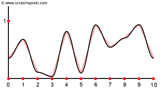
If we use this code, the profile of the curve stays the same (since we are interpolating the same predefined values at the same positions), but the transition between two successive values is much smoother (Figure 8).

Smoothstep

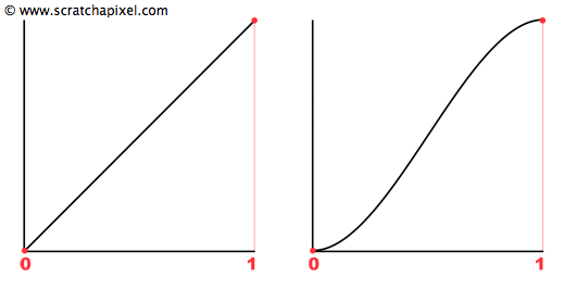
The smooth step function is commonly used in the implementation of noise functions (it is used in the widespread implementation of the noise function written by Ken Perlin, known as Perlin noise). There is nothing much to say about the function itself apart from that its profile (within the range of interest [0:1]) has exactly the shape we are interested in. Here is the equation of the function and its plot (Figure 9, right image. Notice that the Cosine remapping equation ((1-cos(t*M_PI))*0.5) has almost the same profile).

Care must be taken when translating the smoothstep function into code because \(t\) needs to be raised to the power of 2 and 3. It is possible to optimize these operations slightly with the following implementation:

float smoothstepRemap(const float &a, const float &b, const float &t) 
{ 
    float tRemapSmoothstep = t * t * (3 - 2 * t); 
    return Mix(a, b, tRemapSmoothstep); 
} 

Figure 10 shows a plot of the noise function using the smoothstep function. As you can see, it is very similar to the result we got using the cosine function.

A Simple 1D Noise Function

In this lesson section, we will quickly show different ways to change the result of the noise function. First, we will show what our function looks likes. We are still using 10 random numbers to generate our noise pattern (like in Figure 10). This means that our function will vary from 0 to 10 on the x-axis (for values in the range [9:10], we are using the lattices 9 and 0). After that, it will repeat itself with a period of 10 units. We mentioned before that the noise function is a periodic function (Figure 5 illustrates this idea). In real applications, such a short period is not satisfying. Our final version of the noise function will deal with a much larger period (256; we will explain why we use this number). We will also have to write the code to work with negative values for x. We have used the modulo operator to cycle throughout the noise function, but this will not work when x is negative, making it more complicated than it should (and slower). In the final version of the code, you will learn how to handle this case more gracefully. Finally, note how the noise results still vary in the range [0:1] along the y-axis.

Scaling

It is possible to change the shape of the function quite easily by either scaling the input value x or multiplying the result of the function itself. The first operation will change the periodicity of the function. Multiplying x with a value greater than 1 will increase the periodicity of the function (you change the noise function frequency). In short, you will compress the curve (making it appear shorter). This will be more obvious in the next chapter with examples of 2D noise. If we multiply x by a value lower than 1, it stretches the curve out along the x-axis, making it appear longer (Figure 11). This operation is handy for controlling the frequency of the noise pattern.

float frequency = 0.5; 
float freqNoise = valueNoise1D.eval(x * frequency); 

The second most basic operation is multiplying the noise function's result, which changes its amplitude. The effect might be too strong if you use a 1D noise to animate a curve. It can be attenuated by scaling its amplitude down (Figure 12).

float amplitude = 0.5; 
float ampNoise = valueNoise1D.eval(x) * amplitude; 

Offsetting

You can also add a specific value to the input of the noise function. This shifts the curve either to the left (if we add a positive number to x) or to the right (if we add a negative number to x). This technique of shifting the result of the noise function by adding an offset to x is handy for animating the function over time (by increasing the offset value at each frame).

float offset = frameNumber; 
float offNoise = valueNoise1D.eval(x + offset); 

Signed Noise

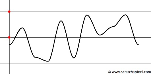
Usually, noise functions return values in the range [0:1]. But it doesn't have to be. It depends on how they are implemented. For instance, you can assign random numbers to the integer lattice point in the range [-1:1], resulting in a noise function returning values in the same range. However, as we said, the convention usually returns a value in the range [0:1], but it is easy enough to remap that value in the range [-1:1]. The resulting noise is sometimes called a signed noise. Here is the code and a plot of our noise function with its result remapped in the range [-1:1] (Figure 21). This can be useful again when you use noise to procedurally animate objects or want to vary a parameter. Imagine that you have an object whose position along the y-axis is 3 and use a signed noise to modulate the object's position along that axis; you might want the object to vary within the range of 0-6. In this case, multiply your signed noise function by 3 so that it varies within the range [-3:3], which, added to 3, will make the object vary within the range [0:6] along the y-axis.

float signedNoise = 2 * valueNoise1D.eval(x) - 1;

A Complete 1D Noise Function

Using ten random numbers results in a very short period. This means the function will repeat itself quite often if we use it over a large range of x values (say from 0 to 100, it will repeat ten times). Visually there is a strong probability that you will be able to spot this pattern, which will not make our result look very natural. We mentioned in the first chapter that one of the noise properties is that it shouldn't look periodic. To achieve this, we will cheat and make the noise function period very large.

In the previous chapter (in the paragraph on the noise properties), we mentioned that when you zoom out enough, the noise becomes so small that a repetition would become hardly visible. This is, in fact, more of a trick than anything else. If you look at the bottom curve from Figure 15, we drew the noise function from 0 to 256 (one period). As you can see, if we were to duplicate this curve to the right and the left and zoom out even more to have a look at these three curves side by side, you probably wouldn't be able to tell that this line is made of three copies of the same curve. The trick is to find a size for the noise period that is long enough to make it impossible to recognize the pattern as you zoom out but short enough that the random value array stays reasonably small (keeping the memory usage consumption low). And 256 or 512 are good values for achieving that result.

Most modern implementations of the noise function use a lattice grid of 256 points (or 512). The 256 value hasn't been chosen by chance. Why 256 and not 255 or 257? Because this number is a power of two (2^8). When we deal with such numbers, we can replace the modulo C operator (%) with a bit operator (&). In the past, programmers preferred arithmetic operations over the % operator, which was slower. Modern processors/compilers handle this very well, so there's no particular need to switch to the & operator apart from the fact that it makes things simpler when x is negative.

#include <bitset> 
using namespace std; 
#define MASK 256 - 1 
int a = -10; 
int b = a & MASK; 
bitset<16> ab(a); 
bitset<16> bb(b); 
bitset<16> mb(MASK); 
cout << ab << "=" << a << "\n" << mb << "=" << MASK << "\n" << bb << "=" << b << "\n"; 
1111111111110110=-10 
0000000011111111=255 
0000000011110110=246

Note how at line 18, we take care of rounding x to the minimum integer value when x is negative (int(-1.2) is -1 while we want -2. So if the boolean test on the right inside is true, then it will add -1 to the result: -1 + -1 = -2). If you are curious and want to check that your function is periodic, then you can write the following code:

template<InterpolationFunc F> 
class ValueNoise1D 
{ 
public: 
    ValueNoise1D(unsigned seed = 2016) 
    { 
        srand48(seed); 
        for (unsigned i = 0; i < kMaxVertices; ++i) { 
            r[i] = drand48(); 
        } 
    } 
 
    // Evaluate the noise function at position x
    float eval(const float &x) 
    { 
        // Floor
        int xi = (int)x - (x < 0 && x != (int)x); 
        float t = x - xi; 
        // Modulo using &
        int xMin = xi & kMaxVerticesMask; 
        int xMax = (xMin + 1) & kMaxVerticesMask; 
 
        return (*F)(r[xMin], r[xMax], t); 
    } 
    static const unsigned kMaxVertices = 256; 
    static const unsigned kMaxVerticesMask = kMaxVertices - 1; 
    float r[ kMaxVertices ]; 
}; 
 
int main(int argc, char **argv) 
{ 
    ValueNoise1D<smoothstep> valueNoise1D; 
 
    static const int numSteps = 200; 
 
    for (int i = 0; i < numSteps; ++i) { 
        // x varies from -10 to 10
        float x = (2 * (i / float(numSteps - 1)) - 1) * 10; 
        std::cout << "Noise at " << x << ": " << valueNoise1D.eval(x) << std::endl; 
    } 
 
    return 0; 
} 

As you can see, calling the noise function with a value for x, a multiple of its period (256), always returns the same value (the value of the random number stored in the array at index 0). You can also write the following code, which is another way of checking the periodicity of the function:

std::cout << valueNoise1D.eval(-512) << std::end; 
std::cout << valueNoise1D.eval(-256) << std::endl; 
std::cout << valueNoise1D.eval(0) << std::endl; 
std::cout << valueNoise1D.eval(256) << std::endl; 
std::cout << valueNoise1D.eval(512) << std::endl; 
 
0.354271 
0.354271 
0.354271 
0.354271 
0.354271 

One Last Very Important Thing to Know

The implementation of the noise function relies on creating an array of random values where each one is considered to be positioned at integer positions on the ruler. This is a very important observation that will be extremely useful when we will come to filtering the noise function later on. In the first chapter of this lesson, we mentioned that when the noise pattern was too small, it became white noise again and created a visual artifact known as aliasing. It is possible to eliminate this aliasing by filtering the noise function when its frequency becomes too high. The question is to know when is "too high". The answer to this question is precisely related to the distance that separates each pre-defined random value on the ruler: two consecutive random numbers are 1 unit apart. You must remember this property of the noise function (a chapter on filtering noise can be found in the lesson Noise Part 2).