Value Noise and Procedural Patterns

Simple Pattern Examples

We will finish this lesson by providing examples of patterns created using the noise function. When Ken Perlin originally developed his noise function, he proposed a few simple algorithms to generate interesting solid textures using this function as a building block. Some of these functions, such as turbulence, are still widely used. He described most of these patterns and a few more in a seminal paper entitled "An Image Synthesiser" which he presented at Siggraph in 1985. This paper can easily be found on the internet, and we highly recommend you read it.

As we said earlier, our version of the noise function doesn't create the most interesting-looking noise (our noise looks quite blocky for now). The goal of this lesson isn't to develop a good-looking noise but to understand how the technique works and the function properties. Check the second Noise Part 2 to learn about a better-looking version of the noise function (called gradient noise, which is the original technique proposed by Ken Perlin in 1985). However, that shouldn't stop us from showing you a few examples, especially with the 2D noise we can use to create more complex patterns. We recommend changing the parameters in the code to understand their effect on the result. In each of the following chapters, you will find a description of the algorithm, the resulting pattern, and the code used to generate the associated image.

1D Noise Examples

One of the first examples we will describe works well in all dimensions. But we will start with the 1D case and give an example later with 2D noise. For a 3D noise example of this technique, look at the second lesson. To sum up, the idea behind it is the contribution of several noises (each layer is often called an octave in the CG literature but avoid this term if possible). We could vary the parameters of these various noise layers (or octaves) - for example, change their frequency and amplitude - in a coherent manner. In other words, we can establish a connection between the change in frequency and amplitude from layer to layer.

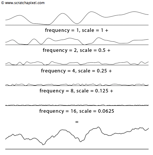
• We will start from a base frequency and unit amplitude (1) and compute the first layer of noise with these values.

• Then, we will add a second layer of noise, but we will multiply the frequency and the amplitude of this layer by 2 and 0.5 (the same as dividing the amplitude by 2), respectively.

• For the third layer, we will multiply the frequency by 4 and divide the amplitude by 4. Layer 4 and 5 will have their frequency and amplitude multiplied by 8 and 16 and divided by 8 and 16, respectively.

If you haven't found the relation yet, each layer is twice the frequency and half the amplitude of the previous layer. If you build a series of noises that way and sum them up together, you get the result from figure 1 (bottom image). As you can see, this curve has a richer profile than a single noise. Visually it looks like the profile of a mountain chain (you can see the concept of octaves or layers as adding up details of smaller frequency to the terrain - since the height of mountains is way greater than the height of rocks making up the fine detail of a landscape, it seems reasonable to decrease the amplitude of the noise layers as their frequency increases). And we are not mentioning this by mistake. As we will show later on with the 2D counterpart of this technique, we can use this result to displace a mesh and create something that looks like a mountain. Remember what we said about noise in the first chapter of this lesson. It can simulate many natural shapes, such as mountains or ocean waves. This is one example.

Before we look a bit more at the terminology, let's say that in this example, a particular layer's frequency and amplitude are driven by a power of two. If we formalize the idea we just described in pseudo-code, we can write:

float noiseSum = 0; 
static const unsigned numLayers = 5;  //octaves 
#if 0 
for (unsigned i = 0; i < numLayers; ++i) { 
    // change in frequency and amplitude
    noiseSum += noise(P * pow(2, i)) / pow(2, i); 
} 
#else 
// alternatively
float amplitude = 1; 
float frequency = 1; 
for (unsigned i = 0; i < numLayers; ++i) { 
    // change in frequency and amplitude
    noiseSum += noise(P * frequency) * amplitude; 
    amplitude *= 0.5;  //1, 0.5, 0.25, 0.0625, ... 
    frequency *= 2;  //1, 2, 4, 8 ... 
} 
#endif 

How many layers shall I use to create this pattern? There is a technical answer that we will only briefly look into. When the frequency of the input value becomes high, the result of the noise function will likely turn into white noise again (see the first chapter of this lesson on noise properties), which we want to avoid. You can sum up as many layers as you want until you reach the point where the frequency of the input value turns the result of the noise function into white noise. This raises another question: do we know when that happens? In theory, yes, we can find out when this happens. This is dictated by the rules of aliasing, a complex and large topic. You will find an explanation about this in the lesson on aliasing and filtering (basic section) and a basic introduction to filtering noise in Noise Part 2.

That's the theory. In practice (when we use this technique for making films), we rarely use more than 3 or 5 layers (sometimes up to 7). There are a couple of reasons for that. First, computing noise is costly. So the more layers you use, the more time you compute. The other main reason is that the layers might not significantly contribute to the result after we have added more than 5 of 7 layers because the amplitude of these layers at that stage becomes small. Should we use more than 5 layers if more layers do not make any significant difference while still expansive to compute (unless you zoom in on the noise pattern)?

Ideally, you want to find a compromise between theory and practice. The perfect code would sum up layers and stop automatically when it finds that the frequency of the input value for the next layer will result in white noise (see the lesson on aliasing for an example of a function that cuts off the number of layers before it turns into white noise). An automatic system could still lead to a very high number of layers, which can be costly. Let the user control the maximum number of layers being used with an input parameter which by default would be set with the values 3, 5, or 7.

Terminology

Some terminology now. The technique of summing up layers of noise in which frequency and amplitude are related can be called a fractal sum. The creation of fractal curves (or surfaces) using this technique is not limited to computer graphics. It looks very similar to a curve that shows the evolution of the stock market over a certain period. These curves and their mathematical representation were studied by Benoit Mandelbrot, a mathematician well known for researching fractal patterns (applied to finance in particular). We will limit ourselves here to introducing a few technical terms. Still, readers interested in this topic can read the lesson on fractals (which is by itself a relatively large and fascinating topic). Many things from the real world, landscapes, seascapes, clouds, and plants, including the evolution of the stock market, etc., have a fractal nature.

When successive layers of a fractal noise have an amplitude inversely proportional to their frequency, the term used to describe the result is pink noise. If we formalize this in a formula, we could write:

float pinkNoise = 0; 
static const unsigned numlayer = 5; 
float rateOfChange = 2.0f; 
for (unsigned i = 0; i < numLayers; ++i) 
{ 
    // change in frequency and amplitude
    pinkNoise += noise(P * pow(rateOfChange, i)) / pow(rateOfChange, i); 
}

More specifically, the change of frequency and amplitude between successive layers almost forms the signature of the resultant noise curve. It defines its spectral properties. We use the term spectral densities to describe the various frequencies (layers) of the resulting noise is made of. And each of these layers has a specific amplitude which we call power spectra. Amplitude and frequency can be related to each other, like in the case of pink noise or not. You could also have a relation in the frequency change between successive layers. These observations are critical to creating many patterns in computer graphics, and we recommend you understand this well before reading any other lessons on pattern creation.

The word noise in the name (pink noise) is misleading as it refers to a sum of noise functions with correlated frequencies and amplitudes. The term octave is also sometimes (mis-)used in place of the word layer. The term layer is more generic than an octave, which is also used in music. An octave is a doubling or halving of a frequency. If it is used in a program (or in literature), it should mean that each successive layer in the computation of a fractal sum is twice the frequency of the previous layer. It means that the term change of rate in our equation would take the value 2. If the frequency ratio between successive layers is different than 2, this term is inaccurate, and the term layer should be used instead. When we double the frequency between layers and the amplitude of these layers is inversely proportional to their frequency, we obtain a particular type of pink noise called Brownian noise (named after the mathematician Robert Brown).

float brownianNoise = 0; 
const unsigned numlayer = 5; 
float rateOfChange = 2.0f; 
for (unsigned i = 0; i < numLayers; ++i) 
{ 
    // change in frequency and amplitude
    brownianNoise += noise(P * pow(rateOfChange, i)) / pow(rateOfChange, i); 
} 

In computer graphics, you will often find that fractal functions are called fBm (which stands for fractional Brownian motion). The CG community has borrowed most of these terms from the mathematics field, mainly as a convenient way of labeling functions using these techniques in a generally simplified/more straightforward form. In the generic form of the fBm function, the amplitude of a layer doesn't have to be inversely proportional to its frequency. You can use two values to control how the frequency and amplitude change between layers. The word lacunarity is used to manage the rate by which the frequency changes from layer to layer. Lacunarity has a special meaning in fractals (check the lesson on fractals for more information). There is no official term to designate the rate of change in the amplitude from layer to layer; in the following pseudo-code of an fBm function, we call it gain:

float fBm(Vec3f P, float lacunarity = 2, float gain = 0.5, int numLayers = 5) 
{ 
    float noiseSum = 0; 
    Vec3f Pnoise = P; 
    float amplitude = 1; 
    for (unsigned i = 0; i < numLayers; ++i) 
    { 
        // change in frequency and amplitude
        noiseSum += noise(Pnoise) * amplitude; 
        Pnoise *= lacunarity; 
        amplitude *= gain; 
    } 
 
    return noiseSum; 
} 

Now that we have established these basic concepts for 1D noise let's see what happens when we apply the same techniques to 2D noise.

2D Noise Examples

To make our program easier, we will first create a simple generic function that will loop all the pixels of an image and compute a 2D position from it. The pixel color is set based on our noise function for that point. This function is a template that takes a noise function as an argument. The noise function is where we will implement the code to compute various patterns (download the source code for a complete example).

template<NoiseFunc N> 
void createNoiseImage(const char *filename) 
{ 
    unsigned imageWidth = 512, imageHeight = 512; 
    float invImageWidth = 1. f / imageWidth; 
    float invImageHeight = 1.f / imageHeight; 
    float noiseFrequency = 5; 
    float *imageBuffer = new float[imageWidth * imageHeight]; 
    float *currPixel = imageBuffer; 
    for (unsigned j = 0; j < imageHeight; ++j) { 
        for (unsigned i = 0; i < imageWidth; ++i) { 
            Vec2f P(i * invImageWidth, j * imvImageHeight) * noiseFrequency; 
            *currPixel = (*N)(P); 
            currPixel++; 
        } 
    } 
    saveImage(filename, imageBuffer, imageWidth, imageHeight); 
    delete [] imageBuffer; 
} 

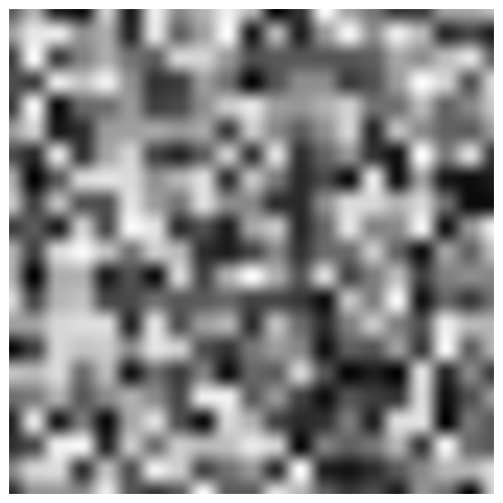
Simple 2D Noise

Our first example is trivial. To demonstrate the use of our program and test our noise function, we first output a simple noise image.

Fractal Sum

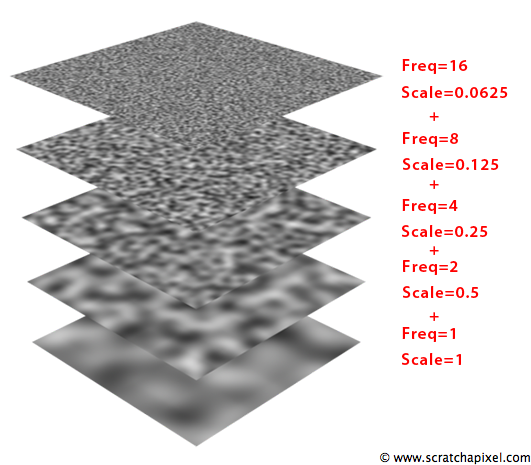
Our second example demonstrates the fractal sum we have already explained for the 1D case. We accumulate the contribution of five layers of noise. Between each successive layer, we multiply the frequency of the point from the previous layer by two and divide the amplitude of the last layer by two.

Here is the resulting image and the code used to compute this result (the code is already slightly optimized. We could have used the function pow(2, k) to change the frequency and amplitude of the noise function. But this function is relatively slow, and we can replace it with a recursive multiplication of the frequency (2) and amplitude (0.5) parameters:

unsigned numLayers = 5; 
float maxNoiseVal = 0; 
for (unsigned j = 0; j < imageHeight; ++j) { 
    for (unsigned i = 0; i < imageWidth; ++i) { 
        Vec2f pNoise = Vec2f(i, j) * frequency; 
        float amplitude = 1; 
        for (unsigned l = 0; l < numLayers; ++l) { 
            noiseMap[j * imageWidth + i] += noise.eval(pNoise) * 2; 
            pNoise *= 2; 
            amplitude *= 0.5; 
        } 
        if (noiseMap[j * imageWidth + i] > maxNoiseVal) maxNoiseVal = noiseMap[j * imageWidth + i]; 
    } 
} 

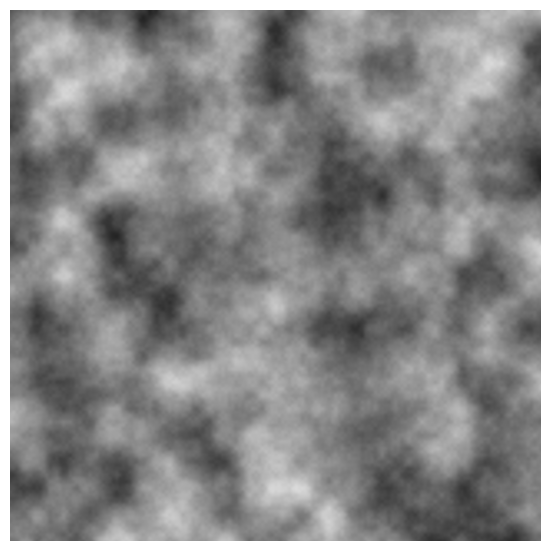
Note that because we sum up several layers of noise, the result could be greater than 1, which will be a problem when we convert this value to a pixel color. We can clamp the value when it is converted to a pixel color. Still, a better solution is to normalize the noise values by dividing all the values in the array by the maximum computed value. To do so, we store the maximum value as we compute all the entries in the noise map in the maxNoiseVal variable. Then once all the values are calculated, we divide them all again by maxNoiseVal (line 12).

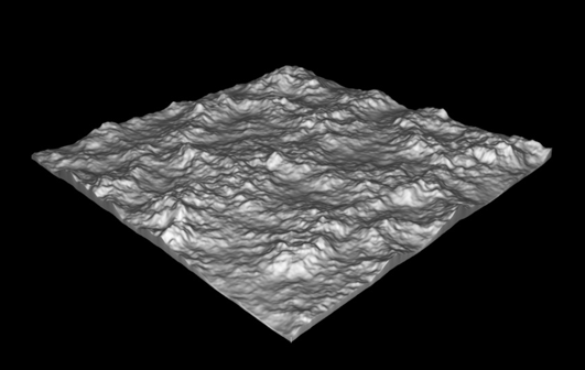
As mentioned, the fractal sum can create convincing terrains and many other natural patterns (seascapes, landscapes, etc.). We can easily create a 2D texture to displace a mesh (Figure 3). More details can be found in the lessons on texture synthesis, terrain generation, and modeling of ocean surfaces.

In the code, you can experiment by changing the frequency and amplitude multiplier, turning your fractal noise function into a more generic fBm function, which we described earlier.

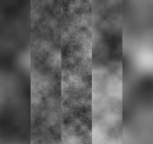
Many different looks can be achieved by varying the value for the lacunarity and the gain, as shown in Figure 4.

ValueNoise noise; 
float frequency = 0.02f; 
float frequencyMult = 1.8;  //lacunarity 
float amplitudeMult = 0.35; 
unsigned numLayers = 5; 
float maxNoiseVal = 0; 
for (unsigned j = 0; j < imageHeight; ++j) { 
    for (unsigned i = 0; i < imageWidth; ++i) { 
        Vec2f pNoise = Vec2f(i, j) * frequency; 
        float amplitude = 1; 
        for (unsigned l = 0; l < numLayers; ++l) { 
            noiseMap[j * imageWidth + i] += noise.eval(pNoise) * amplitude; 
            pNoise *= frequencyMult; 
            amplitude *= amplitudeMult; 
        } 
        if (noiseMap[j * imageWidth + i] > maxNoiseVal) maxNoiseVal = noiseMap[j * imageWidth + i]; 
    } 
} 
for (unsigned i = 0; i < imageWidth * imageHeight; ++i) noiseMap[i] /= maxNoiseVal;

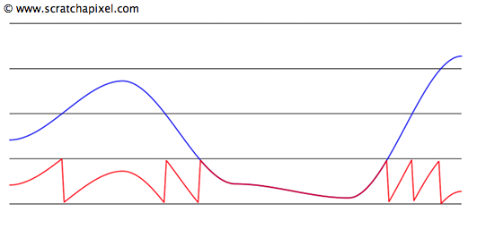
Turbulence

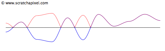
Turbulence is a function built on the same principle as the fractal sum. However, instead of using the noise function directly for each layer, we will use the absolute value of the signed noise. We will first convert the result of the noise into a signed noise, and then take the absolute value of this result. As you can see in the following figure, processing the noise function creates a profile made of bumps. Wherever the curve is negative (black line), we will mirror the curve in these areas along the x-axis. The red line curve is the result. This technique with a 2D noise can produce patterns suitable to simulate fire, smoke, or clouds.

ValueNoise noise; 
float frequency = 0.02f; 
float frequencyMult = 1.8; 
float amplitudeMult = 0.35; 
unsigned numLayers = 5; 
float maxNoiseVal = 0; 
for (unsigned j = 0; j < imageHeight; ++j) { 
    for (unsigned i = 0; i < imageWidth; ++i) { 
        Vec2f pNoise = Vec2f(i, j) * frequency; 
        float amplitude = 1; 
        for (unsigned l = 0; l < numLayers; ++l) { 
            noiseMap[j * imageWidth + i] += std::fabs(2 * noise.eval(pNoise) - 1) * amplitude; 
            pNoise *= frequencyMult; 
            amplitude *= amplitudeMult; 
        } 
        if (noiseMap[j * imageWidth + i] > maxNoiseVal) maxNoiseVal = noiseMap[j * imageWidth + i]; 
    } 
} 
for (unsigned i = 0; i < imageWidth * imageHeight; ++i) noiseMap[i] /= maxNoiseVal;

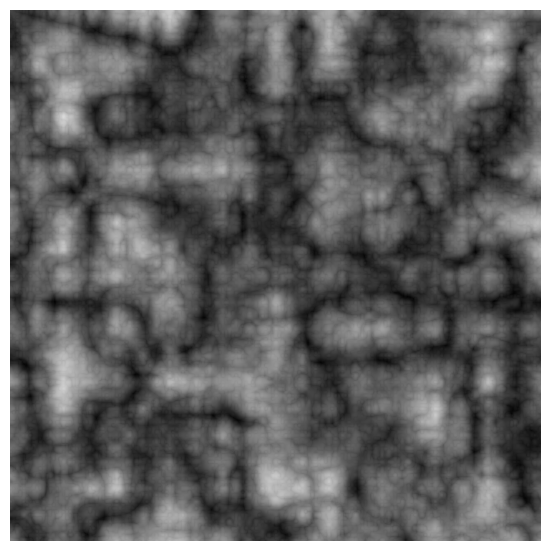
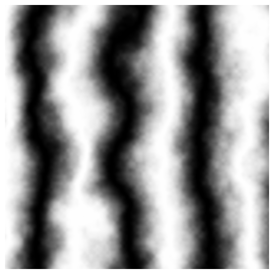
Marble Texture

A marble texture can be created by modulating the phase of the sine pattern with a noise function or a fractal sum. The idea here is not to use the noise function directly to create the pattern but to perturb the function we are using to create the pattern. In that case, we alter or shift the phase of the sine function with a fractal sum. This idea can introduce randomness in any periodic or regular function. Our example is quite simple and only draws a black-and-white marble texture. However, by introducing some color in the mix, it might be possible to create more realistic patterns. The lesson on texture synthesis contains more advanced examples.

float frequency = 0.02f; 
float frequencyMult = 1.8; 
float amplitudeMult = 0.35; 
unsigned numLayers = 5; 
 
Vec2f pNoise = Vec2f(i, j) * frequency; 
float amplitude = 1; 
float noiseValue = 0; 
// compute some fractal noise
for (unsigned l = 0; l < numLayers; ++l) { 
    noiseValue += noise.eval(pNoise) * amplitude; 
    pNoise *= frequencyMult; 
    amplitude *= amplitudeMult; 
} 
noiseMap[j * imageWidth + i] = (sin((i + noiseValue * 100) * 2 * M_PI / 200.f) + 1) / 2.f;

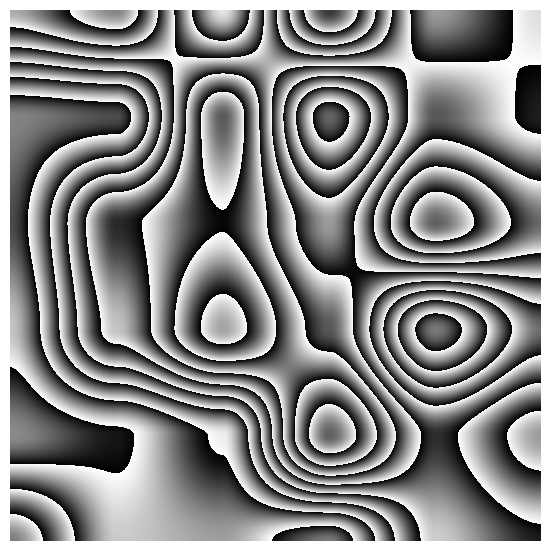
Wood Texture

Like the marble texture, wood relies on a simple trick. The idea is to multiply the noise function by a value greater than 1. Let's call the result of this multiplication \(g\) (historically, it was called \(g\) in reference to wood grain). The texture is obtained by subtracting \(g\) from its integer part. Casting a positive float number to an integer will result in an integer necessarily smaller or equal to \(g\). Therefore, the result of that subtraction is in the range of [0:1) (1 exclusive). Figure 6 illustrates the process. In this example, we have multiplied the noise function by 4. The blue curve represents the value \(g\), while the red curve represents the result of subtracting \(g\) from its integer part. Multiplying the noise function by a value greater than 4 would result in more breakups in the red curve. In 2D, these breakups mark the boundary between regions of lighter and darker color (see the image below).

float g = noise.eval(Vec2f(i, j) * frequency) * 10; 
noiseMap[j * imageWidth + i] = g - (int)g;

References

An Image Synthesizer. Ken Perlin (1985)

Texturing and Modeling, Third Edition: A Procedural Approach. David S. Ebert, F. Kenton Musgrave, Darwyn Peachey, Ken Perlin, Steve Worley (2002)

The Science of Fractal Images, Heinz-Otto Peitgen (1988)