Global Illumination and Path Tracing

An Intuitive Introduction to Global Illumination and Path Tracing

What is Global Illumination Anyway?

Global illumination is simple to simulate. Though, the principal issue with global illumination is that no matter what you do, it is expensive and challenging to simulate efficiently.

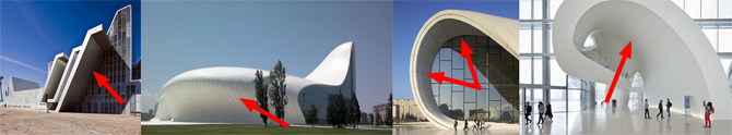
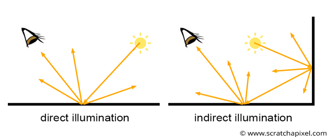
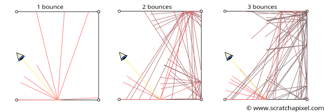
But what is global illumination in the first place, anyway? As you know, we see things because light emitted by light sources, such as the sun, bounces off the objects' surface. When light rays reflect only once from the surface of an object to reach the eye, we speak of direct illumination. But when a light source emits light rays, they more often bounce off of the surface of objects multiple times before reaching the eye (of course, this depends on the schene's configuration). To differentiate this case from direct illumination, we then speak of indirect illumination: light rays follow complex paths while bouncing from object to object before entering our eyes. This effect is visible in the images above. Some surfaces are not exposed directly to light sources (often the sun), yet they are not entirely black. This is because they still receive light because light bounces around from surface to surface.

It is hard to quantify how much indirect illumination accounts for the brightness of a scene. As mentioned before, this depends on the scene's configuration and can thus vary greatly. Still, most often than not, indirect illumination accounts for an essential part of a scene's overall illumination. Simulating this effect is, therefore, of paramount importance if our goal is to produce images close to what we see in (or of) the real world.

Being able to simulate global illumination is a feature that every rendering system should have, so why make a big deal about it? Because while simple in some cases, it is complex to solve generically and also expensive. This explains why for example, most real-time rendering systems don't offer to simulate (at least accurately) global illumination effects.

• It is hard to devise a generic solution that solves all light paths: light rays can interact with many different materials before the eye. For example, a light ray emitted from a light source may be reflected by a diffuse surface first, then travel through a glass of water (it has been refracted then, which means a slight shift or change of direction), then hit a metal surface, then another diffuse surface and then finally hit the eye. There is an infinity of possible combinations. The path a light ray follows from the light source to the eye is called a light path. As you know, light travels from light sources to the eye in the real world. From a mathematical point of view, we know the rules that define how light rays are reflected off the surface of various materials. For example, we know about the law of reflection, refraction, etc. Simulating the path of a light ray as it interacts with various materials is thus something that we can easily do with a computer. Though the problem, as you know, is that forward tracing in computer graphics is not an efficient way of producing an image. Simulating the path of light rays from the light source they are emitted from to the eye is inefficient (see the lesson Introduction to Ray Tracing: a Simple Method for Creating 3D Images if you need a refresher on the subject). We prefer backward tracing which consists of tracing the path of light rays from the eye back to the light source where they originated from. The problem is that backward tracing is an efficient way of computing direct illumination but not always an efficient way of simulating indirect lighting. We will show why in this lesson.

• Direct lighting mainly involves casting shadow rays from the shaded point to the various light sources contained in the scene. How fast computing direct lighting depends on the number of light sources in the scene. Though computing indirect lighting is generally many times slower than computing direct lighting because it requires simulating the path of a great number of additional light rays bouncing around the scene. Generally, simulating these light paths can be more easily done with rays, though ray tracing, as we also know, is quite expensive. As we progress with the lesson, understanding why simulating global illumination is expensive will become more apparent.

How Do We Simulate Indirect Lighting with Backward Tracing

To understand the problem of simulating global illumination with backward tracing, you first need to know how we can simulate indirect lighting. As suggested, many attempts have been made to formalize this process, i.e., putting the process into a mathematical form (interested and mathematically savvy readers can find some information in the reference section at the end of this lesson). Though, we will first explain the process in simple terms.

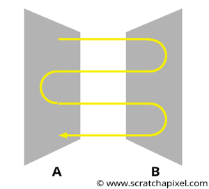
We know from the previous lesson that light illuminating a given point \(P\) on the surface of an object can come from all possible directions contained within a hemisphere oriented about the surface normal \(N\) at \(P\). Finding where light comes from is simple when dealing with direct light sources. We need to loop over all the light sources in the scene and either consider their direction if it is a directional light or trace a line from the light source to \(P\) if the light is a spherical or point light source. Though when we want to account for indirect lighting, every surface above \(P\) may redirect light towards \(P\). Though, as we just mentioned, finding the direction of light rays when dealing with delta lights is simple, how do we do that when a surface emits light? We don't have a single light position from which the light direction can be computed. Since we deal with a surface, there is an infinity of points we could choose on the surface of that object to compute the light direction. Why should we choose one direction rather than another, considering that every point on the surface of that object is likely to reflect light towards \(P\)? And if we choose all the points, there's an infinity of them; thus, this is not a practical choice either.

The answer to this question is both simple and challenging. In some situations, the problem can be solved analytically; there is a closed-form solution to this problem. In other words, it can be solved with an equation. This happens when the shapes of the objects making up the scene are simple (spheres, quads, rectangles), when the objects are not shadowing each other, and have constant illumination across their surface. As you can see, this makes a lot of "ifs". In other words, it is, for example, quite simple to compute the exchange of light energy between two rectangular patches or between a rectangle and a sphere as long as they are not occluded by some other objects and as long as they have a constant color. But as soon as we place a third object between the patch and the sphere or as soon as we shade these objects, then these simple analytical closed-form solutions don't work anymore. For more information on this topic, please check the lessons on rendering in the advanced section (and the lesson on radiosity in particular).

Thus, we must find a more robust solution to this problem in which the solution works regardless of the object's shape and doesn't depend on the object's visibility. Solving this problem with these constraints is pretty hard. We can use a simple method called Monte Carlo integration. The theory behind Monte Carlo integration is explained in great detail in two lessons you can find in the section The Mathematics of Computer Graphics. But why integration? Because, in essence, what we are trying to do is "gather" all light coming from all possible directions above the hemisphere oriented about the normal at \(P\), and this, in mathematics, can be done using what we call an "integral" operator:

\(\Omega\) (the Greek capital letter for omega) here represents the hemisphere of directions oriented about the normal at \(P\). It defines the region of space over which the integral is performed.

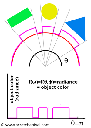
What we integrate is generally a function. So what is that function in our case? In Figure 3, you can see the illumination of \(P\) by other objects in the scene as a function. This function is non-zero in whatever parts of the half-disk onto which objects in the scene are projected (assuming the objects themselves are not black). This function can be parametrized in different ways. It can be a function of solid angle (the Greek letter omega: \(\omega\)) or a function of the spherical coordinates \(\theta\) and \(\phi\) (the Greek letters theta and phi). These are just two different ways (but equally valid) of parametrizing the hemisphere. Considering the 2D case (Figure 3), this can be defined as a function of the angle \(\theta\).

You should start to see how we will solve the "which point on the surface of an object should we choose to compute the contribution of that object to the illumination of my shaded point \(P\)". The fact that we use an integral here and need to gather all light coming from all directions suggests that it's not one point on the surface of that object that we need but all the points making up the surface of that object. Of course, trying to cover the surface of an object with points is not practical or possible. Points are singularities, i.e., they have no area; thus, we can't represent a surface with an infinity of points with no physical size. To solve the problem, one possible solution would be to divide the object's surface into a very large number of tiny patches and compute how much each patch making the surface of that object contributes to the illumination of \(P\). This, in computer graphics, is technically possible and is called the radiosity method. A method exists to solve the problem of light transfer between small patches and \(P\). Still, they have limitations (they are suitable for diffuse surfaces but not for glossy or specular surfaces). More information on the radiosity method can be found in the following sections. Another method would consist of dividing the surface of the objects into small patches and simulating the contribution of these patches to the illumination of \(P\) by replacing them with small point light sources. This would somehow be possible, and an advanced rendering technique called VPL is based on this principle, but Monte-Carlo ray-tracing is simpler and more generic in the end.

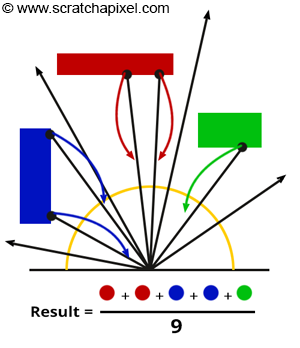
Monte Carlo is another way of solving the problem. It is essentially a statistical method that is based on the idea that you can approximate or estimate how much light is redirected towards \(P\) by other objects in the scene by casting rays from \(P\) in random directions above the surface and evaluating the color of the objects these rays intersect (if they do intersect geometry). The contribution of each of these rays is then summed up, and the resulting sum is divided by the total number of rays. In pseudo-mathematical terms, you can write:

$$\text{Gather Light} \approx \dfrac{1}{N} \sum_{n=0}^N \text{ castRay(P, randomDirectionAboveP) }.$$

This is a quick note for readers already familiar with Monte Carlo integration. You probably already know that the complete equation to compute an approximation of an integral using Monte Carlo integration is:

$$\langle F^N \rangle = \dfrac{1}{N} \sum_{i=0}^{N-1} \dfrac{f(X_i)}{pdf(X_i)}.$$

Suppose you are not familiar with Monte Carlo methods. In that case, you can find them explained in two lessons from the section Mathematics of Computer Graphics. If you look at the equation above, you will notice a PDF term that we will ignore for now, just for the sake of simplicity. We want you to understand the principle of Monte Carlo integration at this point, so don't worry too much about the technical details we will study in the next chapter.

The easiest way of making sense of the Monte Carlo integration method if you have never heard about it before is to think of it in terms of polls. Let's say you want to know the average height of the entire adult population of a country. You can measure each person's height, sum up all the heights and divide this sum by the total number of people. Of course, there are too many people in this population, and it would take too long to do so. We say the problem is intractable. Instead, you measure the height of a small sample of that population, sum up the numbers and divide the sum by the sample size (let's call this number N). The technique works if people making up that sample are chosen randomly and with equiprobability (each individual making up the sample has the same chance to be part of the sample as any other individual making up the population). This is what we call a poll. The result is probably not the exact number, but it is generally a "good" estimation of that number. We are increasing N, increasing (in terms of probability) the quality of your estimation. The principle is the same for approximating or estimating the amount of light reflected towards \(P\) by other objects in the scene. The problem is also intractable because we can't account for all the directions in the hemisphere (as mentioned before, surfaces are continuous, and there's an infinity of points on their surface and therefore an infinity of directions, thus the problem is intractable here as well). Therefore we select a few directions randomly and take the average of their contribution.

Which in pseudo-code translates to:

int N = 16; // number of random directions
Vec3f indirectLigthingApprox = 0;
for (int n = 0; n < N; ++n) {
    // cast a ray above P in a random direction in the hemisphere oriented around N, the surface normal at P
    indirectLigthingApprox += castRay(P, randomDirectionAboveP); // accumulate results
}
// divide by the total number of directions taken
indirectLigthingApprox /= N;

In CG, we call these random directions samples. What we do with Monte Carlo sampling is sampling or taking samples over the domain of the integral or the region of space over which the integral \(\int_\Omega L_i\) is performed, which in this particular case is the hemisphere.

Don't worry about how we choose these random directions over the hemisphere and how many samples (N) we need to use. We will provide more information on this soon. For now, what you need to remember from this part of the lesson, is that the Monte Carlo integration method only provides you with an estimation (or approximation) of the real solution, which is the result of the integral \(\int_\Omega L_i\). The "quality" of this approximation mostly depends on N, the number of samples used. The higher N, the more likely you are to get a result close to the actual result of this integral. We will come back to this topic in the next chapter.

What do we mean by sampling? Since we need to account for the fact that light can come from anywhere above \(P\), what we do instead, in the case of Monte Carlo integration, is to select some random directions within the hemisphere oriented about \(P\) and trace rays in these directions into the scene. Suppose these rays intersect some geometry in the scene. In that case, we then compute the object color at the intersected point which we assume to be the amount of light that the intersected object reflects towards \(P\) along the direction defined by the ray:

Vec3f indirectLight = 0;
int someNumberOfRays = 32;
for (int i = 0; i < someNumberOfRays; ++i) {
    Vec3f randomDirection = getRandomDirectionHemisphere(N);
    indirectLight += castRay(P, randomDirection );
}
indirectLight /= someNumberOfRays;

Remember that we want to collect all light reflected towards \(P\) by objects in the scene, which we can write with the integral formulation: \(\int_\Omega L_i\). The variable \(\Omega\) represents the hemisphere of directions oriented around the normal at \(P\). This is the equation we are trying to solve, and to get an approximation of this integral using Monte Carlo integration, we need to "sample" the function on the right side of the integral sign (the \(\int\) symbol), the \(L_i\) term.

Let's now see how this work with an example. For now, we will work in 2D, but later in the lesson, we will provide the code to apply this technique to 3D.

Let's imagine that we want to compute the amount of light arriving indirectly at \(P\). We first draw an ideal half disk above \(P\) and aligned it along the surface normal at the shaded point. This half disk is just a visual representation of the set of directions over which we need to collect light reflected towards \(P\) by surfaces in the scene. Next, we will compute N random directions, which you can see as N points located on the outer line of the half-disk whose locations on that line are randomly selected. In 2D, this can be done with the following code:

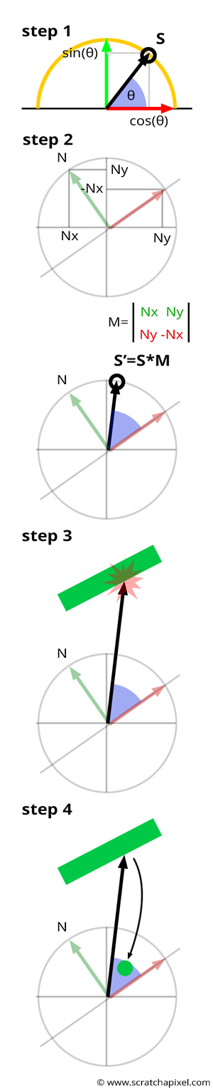
• step 1: what we do is first select a random location in the half disk of the unit circle, which we can do by simply drawing a random value for the angle \(\theta\) anywhere in the range \([0, \pi]\). Computing a random angle can be done using some C++ random function (such as drand48()) which, if it returns a random float in the range \([0,1]\), needs to be correctly remapped to the range \([0, \pi]\).

• step 2: next, notice that the "sampled" direction is located on a half disk that is not yet oriented along the shaded point normal. The best way of doing this is first to construct a 2x2 matrix using the shaded point normal and an interesting property of 2D vectors: a 2D cartesian coordinate system can be created from \((V_x, V_y)\) and from \((V_y, -V_x)\). Both vectors define a Cartesian coordinate system's up and right axes. If you try to apply this technique to any 2D vectors, you will see that the vectors are always perpendicular to each other. Now that we have that matrix, we can rotate our sample directions.

• step 3: we can finally trace a ray in the sampled direction. This step aims to find out if the ray we just sampled hits an object in the scene. If it does, we then compute the color at the point of intersection which we assume to be the amount of light the intersected object reflects towards \(P\) along the ray direction.

• step 4: now that we know how much light is reflected towards \(P\) by an object in the scene along the sample direction, we can treat the result of this intersection as if it was simply a light. In this example, we will assume that the object \(P\) belongs to is diffuse. Thus, we will multiply the object color at the ray intersection point by the cosine of the angle between the surface normal \(N\) and the light direction, which in our case, is the sample direction. We also assume that all other objects in the scene are diffuse (since we call the castRay() function recursively, which on its own only computes the appearance of diffuse surfaces in this example).

• step 5: we accumulate the contribution of the sample.

• step 6: the Monte Carlo integration equation tells us we need to divide the sum of the sample's contribution by the sample size, the number N.

• step 7: we can finally accumulate the diffuse color of the object at \(P\) due to direct and indirect illumination and multiply the sum of these two values by the object albedo (don't forget to divide the diffuse albedo by \(\pi\), the normalizing factor as explained in the introduction on shading).

vec3f castRay(Vec2f P, Vec2f N, uin32_t depth) {
    if (depth > scene->options.maxDepth) return 0;
    Vec2f N = ..., P = ...; // normal and position of the shaded point
    Vec3f directLightContrib = 0, indirectLightContrib = 0;
    // compute direct illumination
    for (uint32_t i = 0; i < scene->nlights; ++i) {
        Vec2f L = scene->lights[i].getLightDirection(P);
        Vec3f L_i = scene->lights[i]->intensity * scene->lights[i]->color;
        // we assume the surface at P is diffuse
        directLightContrib += shadowRay(P, -L) * std::max(0.f, N.dotProduct(L)) * L_i;
    }
    // compute indirect illumination
    float rotMat[2][2] = {{N.y, -N.x}, {N.x, N.y}}; // compute a rotation matrix
    uint32_t N = 16;
    for (uint32_t n = 0; n < N; ++n) {
        // step 1: draw a random sample in the half-disk
        float theta = drand48() * M_PI;
        float cosTheta = cos(theta);
        float sinTheta = sin(theta);
        // step 2: rotate the sample direction
        float sx = cosTheta  * rotMat[0][0] + sinTheta  * rotMat[0][1];
        float sy = cosTheta  * rotMat[1][0] + sinTheta  * rotMat[1][1];
        // step 3: cast the ray into the scene
        Vec3f sampleColor = castRay(P, Vec2f(sx, sy), depth + 1); // trace a ray from P in random direction
        //Steps 4 and 5: treat the returned color as if it was light (we assume our shaded surface is diffuse)
        IndirectLightContrib += sampleColor * cosTheta; // diffuse shading = L_i * cos(N.L)
    }
    // step 6: divide the result of indirectLightContrib by the number of samples N (Monte Carlo integration)
    indirectLightContrib /= N;

    // final result is diffuse from direct and indirect lighting multiplied by the object color at P
    return (indirectLightContrib + directLightContrib) * objectAlbedo / M_PI;
}

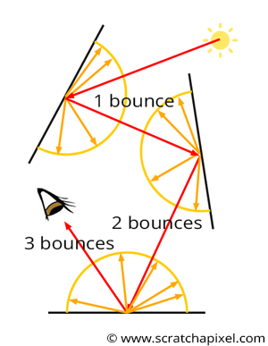
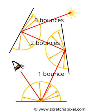
Et voila! You are done. You might see why the technique is expensive, though. When you want to compute indirect illumination (indirect diffuse in this case, as we simulate how diffuse surfaces illuminate each other), you need to shoot many rays (16 in the example above). Every time one of these rays intersects a diffuse surface, you repeat the same process: the process is recursive. After 3 bounces, this is already 16 * 16 * 16 = 4096 rays cast into the scene (assuming all rays intersect geometry). This number increases exponentially as the number of bounces increases. For this reason, as in the case of mirror reflections, we stop casting rays after a certain number of bounces (for example, 3) which in the code above is controlled by the maxDepth variable once again.

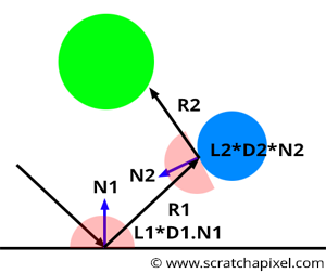
Note that the contribution of a bounce decreases as the ray depth increases. This is because each time a new ray is cast from a surface, its contribution is attenuated by the cosine law. If we consider 2 bounces, for now, a ray is cast in the scene and intersects an object in \(P_1\) (bounce 1). The color at this intersection point \(C_1\) is attenuated by the dot product between the shading normal and the ray direction \(D_1\). Another ray is cast from \(P_1\) and intersects an object in \(P_2\). We then attenuate the contribution of this ray \(R_2\) by the cosine of the angle between the shading normal at \(P_2\) and the ray direction \(R_2\), but the contribution of this ray is itself attenuated again later on by the cosine of the angle between the shading normal at \(P_1\) and the first sample direction \(D_1\). As you can see, the contribution of the second bounce is attenuated twice. The contribution of a third bounce would be attenuated three times, etc. As a result, there is a point where simulating more bounces makes very little difference to the final image (this depends on the scene configuration, but for diffuse surfaces, this is generally the case after 4 or 5 bounces).

Technically, you know how to simulate indirect and indirect lighting, allowing you to create realistic pictures. However, the problem is not that simple. First, in this example, all we have learned to do is to simulate indirect lighting by diffuse surfaces. First, perfect diffuse surfaces rarely exist in nature. But more importantly, most scenes contain a combination of diffuse and specular materials. We didn't even speak yet of other kinds of materials, such as translucent materials, which are not precisely diffuse. Now you may think, why wouldn't Monte Carlo integration work to simulate over kind of materials? It works, but the method reveals itself to be inefficient when the scene contains a mix of specular or transparent and diffuse surfaces. Let's see a few examples.

Using the Indirect Diffuse Sampling Method to Compute Indirect Specular Is Inefficient

There are essentially two kinds of material: specular and diffuse. As explained in the previous lesson, all light sources (direct or indirect) located above a point located on the surface of a diffuse object contribute to the brightness of that point. Of course, the contribution of each light source (again, whether direct or indirect) is attenuated by the cosine of the angle between the light direction and the surface normal, but we will ignore this detail for now. Remember that a diffuse reflection is view-independent. A diffuse surface will always have the same brightness regardless of which angle you look at it. Specular surfaces are different: they are view-dependent. You can only see the reflection of an object if the angle of view is roughly aligned with the mirror reflection along which the light of this object is reflected. This essentially means that light rays reflected by a glossy surface are reflected within a cone of directions oriented about the reflection direction, as explained in the previous chapter. Remember that when we compute the contribution of an object to the illumination of a diffuse object, we speak of indirect diffuse. Similarly, when we want to compute the contribution of an object to the illumination of a glossy object, we speak of indirect specular. Remember two other things:

• For a glossy surface, a beam of light with a given incident direction is reflected in a cone of directions (the specular lobe). How wide that cone depends on the surface roughness. The rougher the surface, the larger the cone.

• Reflection by surfaces is a reciprocal process: swapping the view and the incident direction does not change how a surface reflects light.

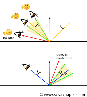
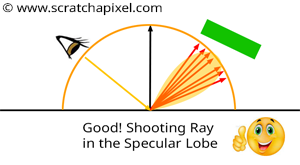
For a diffuse surface, a light always contributes to the illumination of \(P\) regardless of its position (as long as the light is above the surface). For a specular surface, though, a light can only be visible if the view direction \(V\) is roughly aligned with the mirror direction \(R\) of the incident light direction. How close \(V\) and \(R\) have to be, depends on the surface roughness. If the surface is very rough, some light might still be reflected by the surface along the view direction even if \(V\) is not closely aligned with the mirror direction \(R\), as shown in Figure 7 (top). Though as soon as \(V\) is totally outside the cone of directions in which the specular surface reflects light rays, there should be no light reflected at all (Figure 7 - top). We can use this observation to compute the glossy reflection of an object on a glossy surface. If we know the view direction \(V\), then only light rays with specific incident directions will be reflected toward the eyes along \(V\). Now imagine you compute the mirror direction of the vector \(V\) as shown in Figure 7 (bottom). This gives us the vector \(R_V\). Let's now imagine the cone of directions in which light rays are reflected but centered around \(V_R\). What happens? This tells us that any light ray whose incident direction is contained within that cone of direction will somehow be reflected along \(V\) to at least some quantity greater than 0.

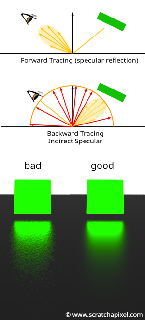
Here is why the technique we used to compute indirect diffuse doesn't work well for indirect specular. We have just explained that only light rays contained within the cone of direction centered around \(V_R\) somehow contribute to the amount of light that is reflected along \(V\). Thus, we should only be interested in the directions within that cone (as shown in Figure 7). The problem with the technique we have used so far, sampling the entire hemisphere, is that many of the created directions are not contained within that cone. Another way of saying this is that because the path of the samples is chosen randomly, there is no guarantee that any of the rays will be contained within the specular lobe's cone of directions at all (Figure 8 - middle). Even if just a few rays are included in this cone, all the rays not contained within the cone itself are somehow wasted anyway since we know that even if they hit an object, their contribution will be null. So the technique is inefficient because many of the rays we cast if we sample the hemisphere are wasted.

This is a quick and simplistic view of what the problem is. Suppose you are already familiar with Monte Carlo integration. In that case, you will understand that, ideally, you want all the samples you use to sample somehow the function that you try to integrate into places where the function is not zero. Doing otherwise will increase what we call variance, which visually translates into what we call noise. You can see the difference in the rendering of the reflection of the green square by a glossy surface in Figure 8. On the left, we can see an example of an image with a lot of noise compared to the image on the right, which seems almost noiseless. However, the two images were rendered with the same number of samples, N. On the left, we have high variance, and on the right low variance. A complete lesson in the next section will explain how this can be done. Many techniques, such as importance sampling, can be used to reduce variance (variance reduction). In the next chapter, you can find more information on noise and the relationship between N, the number of samples used, and the amount of noise in the image.

Your intuition should tell you that the solution to the problem we have just described is to cast rays that are all contained within the specular lobe's cone of directions (Figure 9). Their direction should still be random because this is a requirement of the Monte Carlo integration method, but we should cast them in useful directions. They are different ways of doing so, but we will study them in a lesson on advanced global illumination, which you can find in the next section.

Caustics: The Nightmare of Backward Tracing

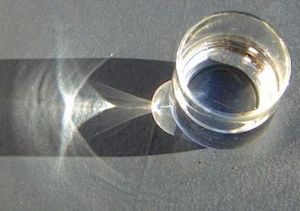
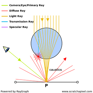
We already talked about the difficulty of simulating caustics in the introduction on light transport. Caustics are the results of light rays being focused in specific points or regions of space by a specular surface or as a result of refraction (light rays passing through a glass of water or wine are focused to a point when then exists the glass as shown in Figure 10 and 11.

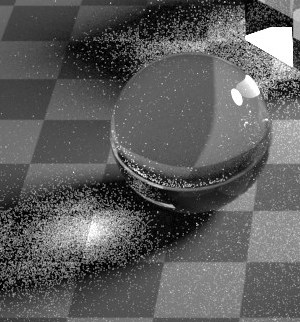
The problem with caustics is similar to the previous issue with distributing samples over the hemisphere to simulate indirect specular reflections. As you can see in Figure 11, many of the rays do not intersect with the sphere, which concentrates all light rays towards \(P\) the shaded point. One ray intersects the sphere but intersects at a point far from the region where light rays are gathered and leave the sphere. Even though \(P\) is likely to be very bright due to many light rays converging to its location, our Monte Carlo method fails to find where in the scene light illuminating \(P\) comes from. As a result, the shaded point will appear dark in the render when it should be quite bright. Simulating caustics creates highly noisy images, as shown in Figure 12.

Caustics are different from indirect specular reflections in that, at least in the case of indirect reflections, we have some prior knowledge of the directions in which we should cast the rays. We said they should be contained with the specular lobe's cone of directions, and we explained why. Though in the case of caustics, we don't know where these caustics are created in the scene. We don't know which parts of the scene concentrate and redirect light rays towards \(P\). Of course, we can increase the number of samples N, but you may need to increase it to a very large number to reduce variance significantly, and this comes at the price of increasing render time greatly. This is not a good solution. A good solution is to decrease variance significantly while keeping render times low.

In reality, there are no reasonable solutions to simulate caustics using backward tracing, which is why the researcher came up with other approaches. One of the most common ones is to simulate light propagation by highly specular and transparent objects from the scene using forward tracing in a pre-pass. After interacting with glossy or refractive materials, light rays hit diffuse surfaces, and their contribution to the point where they hit the diffuse object is stored in a spatial data structure. At render time (after the pre-pass, when we compute the final image), when a diffuse surface is being hit by a primary ray, for instance, we look into this spatial data structure to determine whether some energy was deposited there during the pre-pass by some specular or transparent objects. This is the foundation of a technique called photon mapping, which we will discuss in another section.

More generally, the idea of combining both backward and forward tracing to solve complex light transport provides better results than just using backward or forward tracing alone (in the photon mapping example, we use forward tracing in the pre-pass to follow the path of light rays as they interact with glossy and refractive objects and backward tracing to solve for visibility and direct lighting). This is the approach used by many light transport algorithms such as photon mapping, which we already talked about or bidirectional path tracing, which we will study in the next section. Of course, these other light transport algorithms have their limitations.

What's Next?

We will study and implement in our renderer indirect diffuse using Monte Carlo integration.