Bézier Curve
Reading time: 18 mins.Newell's Teapot

In 1975, computer researcher Martin Newell needed a new 3D model. Very few models were available to the computer graphics community, and creating them took a lot of work. Most models had to get their points entered in the computer program by hand or with a graphics tablet ("a computer input device that allows hand-drawn images and graphics to be input. For example, it may be used to trace an image from a piece of paper laid on the surface. Capturing data in this way is called digitizing"). The story goes that Newell drew a teapot he had at home and digitized these drawings to create the model we know today as the Utah Teapot (figure 1). The teapot is now usually available in rendering or modeling programs along with other geometric primitives, such as spheres, cubes, tori, etc. The walking teapot toys given by Pixar at SIGGRAPH since 2003, in tribute to Newell's work and his iconic teapot, have even become a cult phenomenon (figure 2).

One of the interesting properties of the teapot created by Newell is that the mathematical model used to define the surface of the object is very compact. The teapot contains 32 patches, each represented by 16 points (the original data set contains 28 patches). You might wonder: "how is it possible to create a complex and smooth shape such as the teapot with such few points?". The main idea of the technique is that these 16 points do not define the vertices of polygons as with the polygon mesh we have studied in the previous section. Instead, they represent the control points of something like a grid or lattice that influence the shape of an underlying smooth surface. These points are like magnets that push or pull the underlying surface. Of course, the surface itself doesn't exist as such. To visualize it, we need to calculate it; we do so by combining these 16 control points weighted by some coefficients. Because the creation of the surface is based on equations, it falls under the category of parametric surfaces. The model used by Newell for the teapot (as many other types of parametric surface exist) is called a Bézier surface (or Bézier curve for curves). Pierre Bézier first described it in 1962. The principle of this technique is easier to understand with curves than surfaces. Its application to 3D surfaces, though, is straightforward.
Bézier Curve
To create a Bézier curve, we only need four points. These points are control points defined in 3D space. As with surfaces, the curve itself doesn't exist until we compute it by combining these four points weighted by some coefficients.
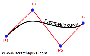
How do we compute this curve? Parametric curves are curves that are defined by an equation. As with every equation, this equation has a variable, which in the case of a parametric curve, is called a parameter. Generally, this parameter is given the letter \(t\). In Figure 4, for example, we have plotted the equation of a parabola \(y=t^2\). As with the parabola example, \(t\) doesn't have to be within any specific range. It can as well go from minus to plus infinity. In the case of a Bezier curve, though, we will only need the value of t going from 0 to 1.

Evaluating the curve's equation for values of \(t\) going from 0 to 1 is the same as walking along the curve. It is essential to understand that \(t\) is a scalar but that the result of the equation for any \(t\) contained in the range [0:1] is a position in 3D space (for 3D curves, and obviously, a 2D point for 2D curves). In other words, if we need to visualize a parametric curve, all we have to do is to evaluate the curve's equation for increasing values of \(t\) at some regular positions (it doesn't have to be though) and connecting the resulting positions in space to create a polygonal path (as illustrated in figure 5).
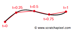
With only four segments, we can see what the overall shape of the curve looks like. All there is to do to get a smoother result is to increase the number of points and segments. This is, in essence, how we will build and visualize Bézier curves. We will sample it at regular intervals and connect the points to create a series of connected line segments. The question now is how do we compute these positions? We mentioned before that shape of the curve was the result of combining the control points weighted by some value (equation 1):
$$P_{curve}(t) = P1 * k_1 + P2 * k_2 + P3 * k_3 + P4 * k_4.$$Where P1, P2, P3, and P4 are the Bézier control points, and \(k_1\), \(k_2\), \(k_3\), \(k_4\) are coefficients (scalar) weighting the contribution of the control points. Looking at figure 3, intuitively, you can see that when \(t\) = 0, the first point on the curve coincides with the control point P1 (for \(t\) = 1, the endpoint coincides with P4). In other words, you can write that:
$$ P_{curve}(t) = \left\{ \begin{array}{ll} P_{curve}(0)= P1 * 1 + P2 * 0 + P3 * 0 + P4 * 0\\ P_{curve}(1)= P1 * 0 + P2 * 0 + P3 * 0 + P4 * 1\\ \end{array} \right. $$Now the parameter \(t\) appears nowhere in these equations. The value of \(t\) is used to compute the coefficients \(k_1\), \(k_2\), \(k_3\), \(k_4\) themselves with the following set of equations (equation 2):
$$ \begin{array}{l} k_1(t) = (1 - t) * (1 - t) * (1 - t)\\ k_2(t) = 3(1 - t)^2 * t\\ k_3(t) = 3(1 - t) * t^2\\ k_4(t) = t^3 \end{array} $$When we need to evaluate a position on the curve for a particular \(t\), we need to replace \(t\) in these four equations to calculate the four coefficients \(k_1\), \(k_2\), \(k_3\), \(k_4\) which are then multiplied to the four control points. That gives us a position in 3D space for a given value of \(t\). For example, if we wish to create a polygon path made of 10 segments, we calculate 11 points by regularly incrementing \(t\) by 1/10. The following code example would calculate these 11 positions along the curve:
int numSegments = 10;
for (int i = 0; i <= numSegments; ++i) {
	float t = i / (float)numSegments;
	// calculate the coefficients
	float k1 = (1 - t) * (1 - t) * (1 - t);
	float k2 = 3 * (1 - t) * (1 - t) * t;
	float k3 = 3 * (1 - t) * t * t;
	float k4 = t * t * t;
	// weight the four control points using coefficients
	point Pt = P1 * k1 + P2 * k2 + P3 * k3 + P4 * k4;
}
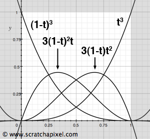
As you can see, the principle is straightforward. All you need to create this curve are four control points which you move around to give the curve the shape you want. Each time you change one of these control points to visualize the new curve, the code above needs to be re-executed. Now that we understand the principle of this method, we will generalize and formalize it. We can formally rewrite the above equation to calculate P (equation 1). You can express it as a sum of control points multiplied by some coefficients:
$$P_{curve}(t)=\sum_{i = 0}^{n} b_{i,n}(t) P_i, \; t \in [0,1]$$The coefficients \(B_{i,n}\) are polynomials ("a polynomial is an expression of finite length constructed from variables and constants, using only the operations of addition, subtraction, multiplication, and non-negative integer exponents") known as the Bernstein polynomials. As you can see from this equation, there are n + 1 coefficients and control points involved in the sum (the sum starts with i = 0 and finishes with i = n, therefore if n = 3, we have i = 0, 1, 2, 3, that is four coefficients).
Bernstein polynomials can be calculated with the following formula:
$$B_{i,n}(t) = \left( \begin{array}{c}n \\ i \end{array} \right)t^i(1-t)^{n-i}, \; i=0,...,n.$$where the terms \(\left( \begin{array}{c}n \\ i \end{array} \right)\) are called binomial coefficients. They can easily be obtained using factorials (the ! sign) with the following equation:
$$\left(\begin{array}{c}n \\ i \end{array} \right) = {n! \over {i!(n - i)! }}$$When n = 3, the binomial coefficients are 1, 3, 3, 1.
The n+1 Bernstein polynomials of degree n (n=3 in our case) form a partition of unity in that they all sum to one.
It is possible to change the value of n (remember that the degree of a polynomial is the largest degree of any one term in this polynomial). Using the Bernstein polynomials, when n = 0, calculating P is equivalent to a linear interpolation:
$$P = (1 - t) * P0 + t * P1$$When n = 2, we say that the Bézier curve is quadratic (\(t\) or \((1-t)\) is raised to the power of 2) and P can be calculated with the following equation:
$$P = (1 - t)^2 * P0 + 2(1-t)t * P1 + t^2 * P2$$When n = 3 (equation 2), we say that the Bézier curve is cubic (\(t\) or \((1-t)\) is raised to the power of 3).
The technique of weighting control points by some coefficients (which are the result of some equations) is widespread in CG. The Bézier curve is perfect for learning about and understanding this technique. It also helps to appreciate how powerful it can be as a mathematical tool. In our particular case, we use it to model a curve in 3D space but imagine that the curve is a function; then, with just a few points and a few coefficients, we would have a compact way of encoding more complex (for example discrete) functions. This is actually how spherical harmonics work (or similar to the principle of DCTs which we explain in the 2D section). The same principle is used for other curves or surface types (such as NURBs).
Bézier Basis Matrix
It is possible to develop the four Bézier basis functions used to calculate the coefficients:
$$ \begin{split} k_1(t) =& (1 - t)^3 = 1 + 3t^2 - 3t - t^3=- t^3 + 3t^2 - 3t + 1\\ k_2(t) =& 3(1 - t)^2t = 3(1 - 2t + t^2)t = 3t - 6t^2 + 3t^3 =\\& 3t^3 - 6t^2 + 3t\\ k_3(t) =& 3(1 - t)t^2 = 3t^2 - 3t^3 = -3t^3 + 3t^2\\ k_4(t) =& t^3 \end{split} $$Remember the algebraic identities: \((a-b)^2=a^2-2ab+b^2\) and \((a-b)^3=a^3 - 3a^2b + 3ab^2 - b^3\). Note that we have ordered the terms from the previous equations by decreasing the exponent value. We can re-write these equations in the form \(ax^3 + bx^2 + cx +d\):
$$ \begin{array}{l} k_1(t) = -1 t^3 + 3t^2 - 3t + 1 \\ k_2(t) = 3t^3 - 6t^2 + 3t + 0\\ k_3(t) = -3t^3 + 3t^2 + 0t + 0\\ k_4(t) = 1t^3 + 0t^2 + 0t + 0 \end{array} $$Finally, we can extract the constants a, b, c, and d from these equations and write them as a 4x4 matrix:
$$\left[\begin{array}{rrrr} -1 & 3 & -3 & 1\\ 3 & -6 & 3 & 0\\ -3 & 3 & 0 & 0 \\ 1 & 0 & 0 & 0\end{array}\right]$$Which we call the Bézier basis matrix. The main idea behind this notation is that the parametric equations can be expressed in the following compact form:
$$\left[\begin{array}{c}t^3 & t^2 & t & 1\end{array}\right]\left[\begin{array}{c}a\\b\\c\\d\end{array}\right]$$This notation is necessary because we can define different types of parametric bicubic curves by changing this matrix's values (examples of such curves are Hermite, BSpline, Catmull-Rom, Bézier). We will develop this topic in a future version of this lesson.
The De Casteljau Algorithm

The De Casteljau algorithm is a numerically more stable way (compared to using the parametric form directly) of evaluating the position of a point on the curve for any given t (it only requires a series of linear interpolations). De Casteljau was one of the first mathematicians to study in the 1950s the possibility of using Bernstein polynomials to construct curves and surfaces (like Bézier, he worked for a car manufacturer and was interested in developing surfacing methods that could be used in CAD software). The principle of the algorithm relies on calculating intermediate positions on each of the three segments defined by the four control points by linearly interpolating the control points for a given t. This process results in three points that can be connected to form two line segments. Next, we repeat the linear interpolation on these two line segments, from which we get two new positions which, again, we can interpolate. The final point from this process lies on the curve at t (this process is illustrated in figure 7). Here is the pseudocode implementing this algorithm:
point decasteljau(point P1, point P2, point P3, point P4, float t)
{
    // calculate the first tree points along main segments P1-P2, P2-P3 and P3-P4
    point P12 = (1 - t) * P1 + t * P2;
    point P23 = (1 - t) * P2 + t * P3;
    point P34 = (1 - t) * P3 + t * P4;
    // calculate the two points along segments P1P2-P2P3 and P2P3-P3P4
    point P1223 = (1 - t) * P12 + t * P23;
    point P2334 = (1 - t) * P23 + t * P34;

    // finally, get P
    return (1 - t) * P1223 + t * P2334; // P
}
Contrary to intuition, maybe, the De Casteljau method is more expensive than evaluating the Bernstein polynomials directly (6 -, 9 +, 22 * for the Bernstein polynomials vs. 6 -, 18 +, 36 * for the De Casteljau method), but as mentioned before, it has proven to be numerically more stable. Furthermore, the De Casteljau algorithm works on curves of arbitrary degree (n=2, n=3, ...) and can be implemented recursively. This is an important point, as initially, this algorithm was developed to recursively subdivide the Bézier curve until some criteria were met (usually to subdivide Bézier curves down to the pixel level and ensure maximum precision when it is displayed on the screen). This technique will be detailed in the lesson on the REYES algorithm (in the advanced section).
Properties of Bézier Curves
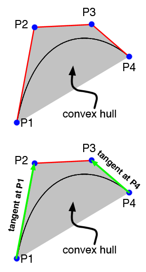
Bézier curves have some interesting properties. We already know that the first and end point of the curve coincides with the first and fourth control point. The lines P1-P2 and P3-P4 are also tangent to the first and end point of the curve. It results from this property that the transition between two Bézier curves is invisible if the line P3-P4 from the first curve is aligned (they are collinear) with the line P1-P2 from the second curve (see figure 8). This property can either extend an existing Bezier curve (by joining several curves together) or split an existing curve in two (see further down). Finally, the convex hull (defined by the control points) of the Bézier polygon contains the Bézier curve (see figure 8).
Connecting and Splitting Bezier Curves
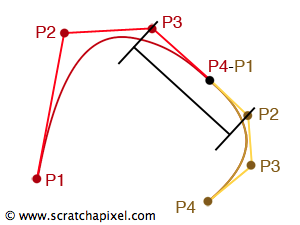
Several Bézier curves can be connected. A 0th order continuity means that the curves are only joined (the last and first points of the first and second curves do join) but are not tangent. 1st order continuity means that the points join and the curves are tangent at the intersection point. 2nd order continuity is possible assuming more constraints on the alignments of the control points (but are more complex to implement, particularly as the degree of the curve (the value of n) increases).

If two Bézier curves can be connected with 1st order continuity (if the last two and first two control points of the first and second point are collinear), then it is also possible to divide a Bézier curve into two sub-curves (which are also Bézier curves). The technique to split the curve relies on the De Casteljau algorithm presented above. If you look at the final image of the animation in figure 7 (which we have reproduced in figure 10), it is intuitively possible to see that two sub-curves can be built from the points P1, P12, P1224, and P for the first sub-curve and P, P2334, P34 and P4 for the second sub-curve. Adapting the pseudocode implementing the De Casteljau method to generate the control points for these two sub-curves is straightforward (the function takes four points for the original input curve and two series of four points for the two generated curves):
point splitBezier(point P[4], float t, point P1[4], point P2[4])
{
    // calculate the first tree points along main segments P1-P2, P2-P3 and P3-P4
    point P12 = (1 - t) * P[0] + t * P[1];
    point P23 = (1 - t) * P[1] + t * P[2];
    point P34 = (1 - t) * P[2] + t * P[3];
    // calculate the two points along segments P1P2-P2P3 and P2P3-P3P4
    point P1223 = (1 - t) * P12 + t * P23;
    point P2334 = (1 - t) * P23 + t * P34;
    // finally, get P
    point P = (1 - t) * P1223 + t * P2334;
    P1[0] = P[0], P1[1] = P12, P1[2] = P1223, P1[3] = P;
    P2[0] = P, P2[1] = P2334, P2[2] = P34, P3[3] = P4;
}
It can be beneficial to recursively split a curve until the resulting sub-curves are considered small enough. For example, if we chose to split the curve at t = 0., five then we can optimize the De Casteljau algorithm slightly and write (substituting 0.5 for t in the previous code and arranging the terms):
point splitBezierOptimize(point P[4], point P1[4], point P2[4])
{
    P1[0] = P[0],
    P1[1] = (P[0] + P[1]) / 2;
    P1[2] = (P[0] + 2P[1] + P[2]) / 4;
    P1[3] = P2[0] = (P[0] + 3(P[1] + P[2]) + P[3]) / 8;
    P2[1] = (P[3] + 2P[2] + P[1]) / 4;
    P2[2] = (P[2] + P[3]) / 2;
    P2[3] = P[3];
}
Interactive Applet
To better understand how Bézier curves work, we wrote a small interactive 2D applet that allows you to see how the shape of the curve changes as you move the control points around. You can randomize the position of the control points using the 'r' key. Note that by default, we use seven control points. You can interpret this configuration as two Bézier curves where the last point of the first curve and the first point of the second curve are the same. When the control points P2, P3, and P4 are aligned, we have a curve with 1st-order continuity at P3 (the curve appears smooth at this point. It has no break). The two curves are C1 continuous at the joining point. If you move P2 or P4soy that P2, P3, and P4 are not aligned anymore (you can alternatively move P3), note how a break appears at P3\. With seven control points, we can interpret the curve as a curve with three points (P0, P3, and P6) and three tangents if P2, P3, and P4 are aligned or four tangents if they are not (we say the tangents are broken at P3). To modify the length and the orientation of these tangents, you can change the position of points P1, P2, P4, and P5. You can force the tangents P2-P3 and P3-P4 to be unbroken by forcing P2, P3, and P4 to stay aligned when you move any of these three points. Of course, you can keep adding more points to create longer curves or more complex shapes.
Alternatively, if you find it too complicated to play with so many points, you can use the 'm' key to only display the first four points of the curve. This would be the most straightforward Bézier curve you could draw (one with only four points). Typing 'm' again will switch back to the seven control points example.
+++
+++
What's Next?
Extending the principle of Bézier curves to surfaces is straightforward and will be the topic of our next chapter.