Rendering Curves as Geometry: Hair Rendering
Reading time: 12 mins.How Do I Render Curves?
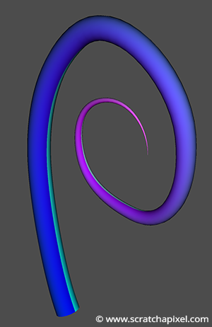
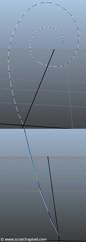
After we wrote the lesson on Bézier curves and surfaces, someone sent us a question regarding ways of rendering 3D Bézier curves as geometry. If you have access to some graphics API (OpenGL, DirectX, WebGL, etc.), you can probably create a 3D window and display a 3D curve as a series of short lines. Though, of course, an alternative solution to this approach is to somehow represent the curve with some 3D geometry that can also be rendered. The two most common approaches to this problem are:
-
Ribbons: the idea of a ribbon is simple, you create a strip of quads along the curve. The geometry created looks like a ribbon, of course, that is, a flat surface. The problem with this approach is often to define what the normal of these quads should be and how the quads should be oriented. You have several options, but the most common one is often to have the quads' normal facing the camera.
-
Thin cylinder or surface of circular cross-section or string of spaghetti (as described in the RIS documentation): in this particular case, we render the curve as a cylinder or round tube following the shape of the curve (as shown in the rendered image above). Like a hose, if you prefer. In this particular approach, note that we generate more geometry than with a ribbon (the geometry is likely to contain more polygons). Still, there is also no problem with the normal orientation.
Both approaches are particularly well suited anyway to render things such as hair, fur or grass and this is why we thought it would be great to have a chapter dedicated to this topic, even if we plan to write a lesson mainly devoted to the subject of hair rendering in the future (at least we hope this short introduction will satisfy your curiosity in the meantime).
We won't show the ribbon solution in this chapter. We will only focus on the second option though it is much simpler to implement the first option from the second than the other way around. So let's do it, shall we?
Step 1: Create Positions at Regular Intervals
What do we need? We first need to create loops of vertices along the curve and then connect these vertices to make faces. First, we know how to create a 3D position along the curve. In our example, we will use a Bézier curve with more than 4 points. We need to compute how many curves we have from the number of input control points, then iterate over each one of these curves, and finally "walk" along the current curve to create a series of 3D positions at regular intervals. We will also compute the tangent at the point, which we will need in step 2 to create a local coordinate system.
constexpr uint32_t curveNumPts = 22;
Vec3f curveData[curveNumPts] = {
    {-0.0029370324, 0.0297554422, 0},
    ...
    { 0.7606914144, 1.7038639600, 0}
};

void createCurveGeometry()
{
    uint32_t ndivs = 16;
    uint32_t ncurves = 1 + (curveNumPts - 4) / 3;
    Vec3f pts[4];
    for (uint32_t i = 0; i < ncurves; ++i) {
        for (uint32_t j = 0; j < ndivs; ++j) {
            pts[0] = curveData[i * 3];
            pts[1] = curveData[i * 3 + 1];
            pts[2] = curveData[i * 3 + 2];
            pts[3] = curveData[i * 3 + 3];
            float s = j / (float)ndivs;
            Vec3f pt = evalBezierCurve(pts, s);
            Vec3f tangent = derivBezier(pts, s).normalize();
        }
        ...
    }
    ...
}
Step 2: Create a Local Coordinate System to Generate a Loop of Vertices
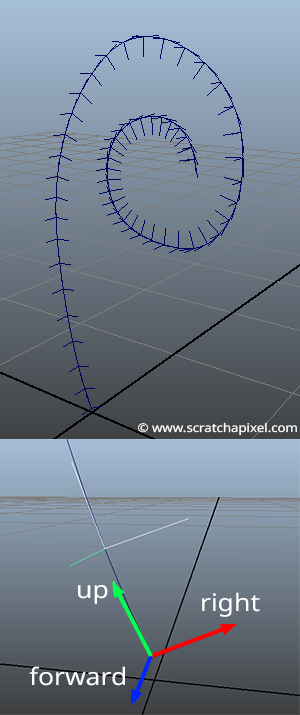
In step 2, we will create a local coordinate system which we will need in step 3, to create a loop of points that will later become the vertices of our thin cylinder. What we want is for all the points of that loop to be lying on a plane perpendicular to the curve tangent. So far, we know the tangent of the curve at a given sampled point. From this tangent, we can create a Cartesian coordinate system. The challenge, though, is that we need to keep this Cartesian coordinate system consistently oriented along the curve to easily connect the vertices to each to form faces in steps 3 and 4. This can be quickly done by always taking the same "random" vector as a starting point and using the trick described in the lesson on geometry, which consists of first computing the cross product between our vector \(v\) and a random vector \(r\). This will give us a vector \(u\) perpendicular to \(v\). Then by taking the cross product between \(u\) and \(v\), we can create a third vector \(w\) which is both perpendicular to \(u\) and \(v\). The three vectors \(u\), \(v\), and \(w\) will then form a Cartesian coordinate system.
Let's always take the tangent along the curve as the up vector of our coordinate system and always choose a consistent vector for \(r\). We can create a series of consistent Cartesian coordinate systems along the curve, as shown in figure 3. Though, note that the way we chose \(r\) depends on the y-coordinate of the tangent or up vector. We choose \(r\) to be as different as possible from the tangent vector. So we first find out which one of the tangent coordinates has the highest value and choose \(r\) accordingly (lines 9 to 38 in the code below).
void createCurveGeometry()
{
    ...
    for (uint32_t i = 0; i < ncurves; ++i) {
        for (uint32_t j = 0; j < ndivs; ++j) {
            ...
            Vec3f tangent = derivBezier(pts, t).normalize();

            uint8_t maxAxis;
            if (std::abs(tangent.x) > std::abs(tangent.y))
                if (std::abs(tangent.x) > std::abs(tangent.z))
                    maxAxis = 0;
                else
                    maxAxis = 2;
            else if (std::abs(tangent.y) > std::abs(tangent.z))
                    maxAxis = 1;
            else
                maxAxis = 2;

            Vec3f up, forward, right;

            switch (maxAxis) {
                case 0:
                case 1:
                    up = tangent;
                    forward = Vec3f(0, 0, 1);
                    right = up.crossProduct(forward);
                    forward = right.crossProduct(up);
                    break;
                case 2:
                    up = tangent;
                    right = Vec3f(0, 0, 1);
                    forward = right.crossProduct(up);
                    right = up.crossProduct(forward);
                    break;
                default:
                    break;
            };

            ...
        }
    }
    ...
}
Step 3: Generate a Loop of Vertices
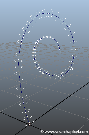
The next step involves creating loops of points correctly oriented around the curve. We will first create a ring of points using basic trigonometry (in the x-z plane of the world coordinate system) and then use the Cartesian coordinate system to transform the point to their final position. Remember that a transformation matrix is more than just the tree vectors representing the axes of a coordinate system. If we apply the equation of point-matrix multiplication, our points should be appropriately oriented (they will lie in the x-z plane of the Cartesian coordinate system). All there is left to do is add or translate the points' position along the curve to move them to their final position along the curve. We also want the cylinder to get thinner as we get closer to the tip of the curve. For this purpose, we compute a normalized (in the range [0:1]) parametric position along the curve (line 7). This value is then used to scale the points' position (lines 8 and 11). We also set the normal of the points (which we will then become the vertices of cylinder mesh), which is simply the position of the transformed points (without the translation - line 16). Don't forget to normalize them. Here is the code:
void createCurveGeometry()
{
    ...
    for (uint32_t i = 0; i < ncurves; ++i) {
        for (uint32_t j = 0; j < ndivs; ++j) {
            ...
            float sNormalized= (i * ndivs + j) / float(ndivs * ncurves);
            float rad = 0.1 * (1 - sNormalized);
            for (uint32_t k = 0; k <= ndivs; ++k) {
                float t = k / (float)ndivs;
                float theta = t * 2 * M_PI;
                Vec3f pc(cos(theta) * rad, 0, sin(theta) * rad);
                float x = pc.x * right.x + pc.y * up.x + pc.z * forward.x;
                float y = pc.x * right.y + pc.y * up.y + pc.z * forward.y;
                float z = pc.x * right.z + pc.y * up.z + pc.z * forward.z;
                P[i * (ndivs + 1) * ndivs + j * ndivs + k] = Vec3f(pt.x + x, pt.y + y, pt.z + z);
                N[i * (ndivs + 1) * ndivs + j * ndivs + k] = Vec3f(x, y, z).normalize();
                st[i * (ndivs + 1) * ndivs + j * (ndivs + 1) + k] = Vec2f(sNormalized, t);
            }
        }
    }
    ...
}
Step 4: Meshing
In the final step, we will connect the vertices to form the faces of the mesh. This is a bit of logic, which doesn't require much explanation. You need to get it right. We need to create an array of integers in which we store the number of vertices each face in the mesh is made of. All the faces are quads apart from the last row of faces in the mesh at the tip of the curves, which are triangles. The strip of triangles at the end of the curve forms a cone whose apex is simply the last point of the curve. Generating the st coordinates for that mesh isn't complicated. All you need to do is set the normalized parametric position along the curve as the vertex's s-coordinate and the vertex's parametric position in the ring as its t-coordinate. Images below show the result of the meshing and the vertex normals for ndivs = 8.
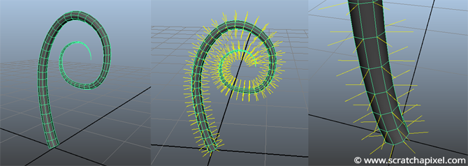
Here is the code of the complete and final function:
void createCurveGeometry()
{
    uint32_t ndivs = 8;
    uint32_t ncurves = 1 + (curveNumPts - 4) / 3;
    Vec3f pts[4];
    std::unique_ptr<Vec3f []> P(new Vec3f[(ndivs + 1) * ndivs * curves + 1]);
    std::unique_ptr<Vec3f []> N(new Vec3f[(ndivs + 1) * ndivs * ncurves + 1]);
    std::unique_ptr<Vec2f []> st(new Vec2f[(ndivs + 1) * ndivs * ncurves + 1]);
    for (uint32_t i = 0; i < ncurves; ++i) {
        for (uint32_t j = 0; j < ndivs; ++j) {
            pts[0] = curveData[i * 3];
            pts[1] = curveData[i * 3 + 1];
            pts[2] = curveData[i * 3 + 2];
            pts[3] = curveData[i * 3 + 3];
            float s = j / (float)ndivs;
            Vec3f pt = evalBezierCurve(pts, s);
            Vec3f tangent = derivBezier(pts, s).normalize();

            uint8_t maxAxis;
            if (std::abs(tangent.x) > std::abs(tangent.y))
                if (std::abs(tangent.x) > std::abs(tangent.z))
                    maxAxis = 0;
                else
                    maxAxis = 2;
            else if (std::abs(tangent.y) > std::abs(tangent.z))
                    maxAxis = 1;
            else
                maxAxis = 2;

            Vec3f up, forward, right;

            switch (maxAxis) {
                case 0:
                case 1:
                    up = tangent;
                    forward = Vec3f(0, 0, 1);
                    right = up.crossProduct(forward);
                    forward = right.crossProduct(up);
                    break;
                case 2:
                    up = tangent;
                    right = Vec3f(0, 0, 1);
                    forward = right.crossProduct(up);
                    right = up.crossProduct(forward);
                    break;
                default:
                    break;
            };

            float sNormalized = (i * ndivs + j) / float(ndivs * ncurves);
            float rad = 0.1 * (1 - sNormalized);
            for (uint32_t k = 0; k <= ndivs; ++k) {
                float t = k / (float)ndivs;
                float theta = t * 2 * M_PI;
                Vec3f pc(cos(theta) * rad, 0, sin(theta) * rad);
                float x = pc.x * right.x + pc.y * up.x + pc.z * forward.x;
                float y = pc.x * right.y + pc.y * up.y + pc.z * forward.y;
                float z = pc.x * right.z + pc.y * up.z + pc.z * forward.z;
                P[i * (ndivs + 1) * ndivs + j * (ndivs + 1) + k] = Vec3f(pt.x + x, pt.y + y, pt.z + z);
                N[i * (ndivs + 1) * ndivs + j * (ndivs + 1) + k] = Vec3f(x, y, z).normalize();
                st[i * (ndivs + 1) * ndivs + j * (ndivs + 1) + k] = Vec2f(sNormalized , t);
            }
        }
    }
    P[(ndivs + 1) * ndivs * ncurves] = curveData[curveNumPts - 1];
    N[(ndivs + 1) * ndivs * ncurves] = (curveData[curveNumPts - 2] - curveData[curveNumPts - 1]).normalize();
    st[(ndivs + 1) * ndivs * ncurves] = Vec2f(1, 0.5);
    uint32_t numFaces = ndivs * ndivs * ncurves;
    std::unique_ptr<uint32_t []> verts(new uint32_t[numFaces]);
    for (uint32_t i = 0; i < numFaces; ++i)
        verts[i] = (i < (numFaces - ndivs)) ? 4 : 3;
    std::unique_ptr<uint32_t []> vertIndices(new uint32_t[ndivs * ndivs * ncurves * 4 + ndivs * 3]);
    uint32_t nf = 0, ix = 0;
    for (uint32_t k = 0; k < ncurves; ++k) {
        for (uint32_t j = 0; j < ndivs; ++j) {
            if (k == (ncurves - 1) && j == (ndivs - 1)) { break; }
            for (uint32_t i = 0; i < ndivs; ++i) {
                vertIndices[ix] = nf;
                vertIndices[ix + 1] = nf + (ndivs + 1);
                vertIndices[ix + 2] = nf + (ndivs + 1) + 1;
                vertIndices[ix + 3] = nf + 1;
                ix += 4;
                ++nf;
            }
            nf++;
        }
    }

    for (uint32_t i = 0; i < ndivs; ++i) {
        vertIndices[ix] = nf;
        vertIndices[ix + 1] = (ndivs + 1) * ndivs * ncurves;
        vertIndices[ix + 2] = nf + 1;
        ix += 3;
        nf++;
    }
}
You can see the result of the mesh being rendered in a ray tracer at the top of this chapter. You can also find the complete source code in the last chapter of this lesson.