Bézier Curves and Surfaces

Calculating Normals of Bézier Surfaces

Reading time: 7 mins.

**Figure 1:** a face normal can be computed from the cross product between two edges of a face.

Now that we studied a couple of techniques to create a Bézier patch, a problem remains. We need to shade this patch. Generating the position of the points is something we can already do for shading, but we also need a normal. How can we generate a normal at the position of each vertex of the grid? We can easily generate a face normal using a technique similar to the one we have used in the getSurfaceProperties method of the TriangleMesh class. We can compute the cross-product between two edges making up a face. But this technique only produces a face normal.

// face normal
const Vec3f &v0 = P[k]; 
const Vec3f &v1 = P[k+1]; 
const Vec3f &v2 = P[k+3]; 
faceNormal = (v1 - v0).crossProduct(v2 - v0);

**Figure 2:** a normal at any point on the patch can be computed from a cross product between the tangent on the surface at that point along the $u$ and the $v$ direction.

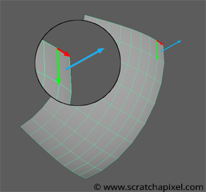
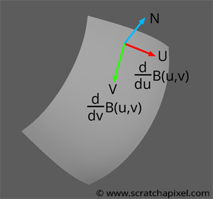
What we want is a vertex normal, a normal at each point making up the grid that is perpendicular to the Bézier surface. Hopefully, because the grid is computed from equations, we can also use maths to calculate an accurate normal at any point on the surface of the Bézier patch. What we want to do is compute two tangents at the point of interest (whose coordinates on the patch are specified in terms of $u$ and $v$), one along the $u$ direction and one along the $v$ direction. By taking the cross-product of these two tangents, we get the normal we are looking for. The question now is, how do we compute these tangents? As suggested, we can express the problem in mathematical terms. In mathematics, the tangent of a curve calculated from a function can be defined as the function derivative with respect to a parameter, for example:

$$\dfrac{\partial}{\partial x}f(x),$$

would represent the derivative of the function $f(x)$ with respect to the parameter $x$. We can do the same thing with the equation to compute points on a Bézier patch. We can, for example, compute the derivative of that function or equation with respect to the parameter $u$ or $v$:

$$\dfrac{\partial}{\partial u}B(u,v), \dfrac{\partial}{\partial v}B(u,v).$$

The first equation would give us a tangent along the $u$ direction, and the second, the tangent along the $v$ direction. Now we know that the function $B(u,v)$ itself can be written as:

$$B(u,v) = \sum_i\sum_j b_i(u) b_j(v) p_{ij}.$$

Where $b_i(u)$ and $b_j(v)$ are the Bernstein polynomials and $p_{ij}$ the control points. We also know how to compute the Bernstein polynomials:

$$ \begin{array}{l} k_1(t) = (1 - t)^3\\ k_2(t) = 3t(1 - t)^2\\ k_3(t) = t^23(1 - t)\\ k_4(t) = t^3 \end{array} $$

So all we need to do is compute the derivative of these functions, which are:

$$ \begin{array}{l} k'_1(t) = -3(1-t)^2\\ k'_2(t) = 3(1-t)^2-6t(1-t)\\ k'_3(t) = 6t(1-t)-3t^2\\ k'_4(t) = 3t^2 \end{array} $$

The derivative of a function of a function such as $(x^2+3)^3$ can be computed using what we call the chain rule.

$$\dfrac{d}{dx}y = \dfrac{d}{du}y \dfrac{d}{dx}u.$$

You need to:

Recognise $u$ (always choose the inner-most expression, usually the part inside brackets or under the square root sign)
Then we need to re-express $y$ in terms of $u$
Then we differentiate $y$ with respect to $u$, then we re-express everything in terms of $x$
The next step is to find $\dfrac{d}{dx}u$
Then we multiply $\dfrac{d}{du}y$ and $\dfrac{d}{dx}u$.

In our example, we let $u = x^2 + 3$ and then $y = u^3$. We see that $u$ is a function of $x$ and $y$ is a function of $u$. For the chain rule, we firstly need to find $\dfrac{d}{du}y$ and $\dfrac{d}{dx}u$.

$$\dfrac{d}{du}y = 3u^2 = 3(x^2 + 3)^2,$$

and:

$$\dfrac{d}{dx}u = 2x.$$

So:

$$\dfrac{d}{dx}y=\dfrac{d}{du}y \dfrac{d}{dx}u=3(x^2 + 3)^2(2x)=6x(x^2+3).$$

If you follow these steps, you will easily find the derivatives of our equations.

If we derive the equation $B(u,v) = \sum_i\sum_j b_i(u) b_j(v) p_{ij}$ with respect to $u$, you will get (this would give us the tangent on the patch for the pair of parameter $(u,v)$ along the $u$ direction):

$$ \begin{array}{l} \dfrac{\partial}{\partial u}B(u,v) =&-3(1-u)^2 \sum_j b_j(v) p_{0j}\\ &3(1-u)^2-6u(1-u) \sum_j b_j(v) p_{1j}\\ &6u(1-u)-3u^2 \sum_j b_j(v) p_{1j}\\ &3u^2 \sum_j b_j(v) p_{3j} \end{array} $$

What we do there is to compute a Bézier parallel to the $u$ direction, and then once we have this curve, calculate the derivative along this curve using $k'_1(u)$, $k'_2(u)$, $k'_3(u)$ and $k'_4(u)$. The same thing can be done to find the tangent along the $v$ direction:

$$ \begin{array}{l} \dfrac{\partial}{\partial v}B(u,v) =&-3(1-v)^2 \sum_i b_i(u) p_{i0}\\ &3(1-v)^2-6v(1-v) \sum_i b_i(u) p_{i1}\\ &6v(1-v)-3v^2 \sum_i b_i(u) p_{i2}\\ &3v^2 \sum_i b_i(u) p_{i3} \end{array} $$

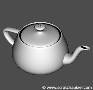
Et voila! All there is left to do is compute these two equations to obtain the two tangents at the parametric coordinates $(u,v)$ and then compute the cross-product between these two tangents to get the normal at this point. The implementation of this technique is shown below. We have two functions, dUBezier to compute the tangent along the $u$ direction and dVBezier to compute the other tangent along the $v$ direction. The result is surprising. As you can see in the adjacent image, the result is not only very smooth but also that the transition at the patches boundaries is invisible. Mathematics once again works remarkably well and gives us a perfect result, including at the edges or corners of the patches.

Vec3f dUBezier(const Vec3f *controlPoints, const float &u, const float &v) 
{ 
   Vec3f P[4]; 
   Vec3f vCurve[4]; 
   for (int i = 0; i < 4; ++i) { 
       P[0] = controlPoints[i]; 
       P[1] = controlPoints[4 + i]; 
       P[2] = controlPoints[8 + i]; 
       P[3] = controlPoints[12 + i]; 
       vCurve[i] = evalBezierCurve(P, v); 
   } 
 
   return -3 * (1 - u) * (1 - u) * vCurve[0] + 
       (3 * (1 - u) * (1 - u) - 6 * u * (1 - u)) * vCurve[1] + 
       (6 * u * (1 - u) - 3 * u * u) * vCurve[2] + 
       3 * u * u * vCurve[3]; 
} 
 
Vec3f dVBezier(const Vec3f *controlPoints, const float &u, const float &v) 
{ 
   Vec3f uCurve[4]; 
   for (int i = 0; i < 4; ++i) { 
       uCurve[i] = evalBezierCurve(controlPoints + 4 * i, u); 
   } 
 
   return -3 * (1 - v) * (1 - v) * uCurve[0] + 
       (3 * (1 - v) * (1 - v) - 6 * v * (1 - v)) * uCurve[1] + 
       (6 * v * (1 - v) - 3 * v * v) * uCurve[2] + 
       3 * v * v * uCurve[3]; 
} 
 
void generatePolyTeapot(const Matrix44f& o2w, std::vector<std::unique_ptr<object>> &objects) 
{ 
   uint32_t divs = 8; 
   ... 
   Vec3f controlPoints[16]; 
   for (int np = 0; np < kTeapotNumPatches; ++np) {  //kTeapotNumPatches 
       // set the control points for the current patch
       for (uint32_t i = 0; i < 16; ++i) 
           controlPoints[i][0] = teapotVertices[teapotPatches[np][i] - 1][0], 
           controlPoints[i][1] = teapotVertices[teapotPatches[np][i] - 1][1], 
           controlPoints[i][2] = teapotVertices[teapotPatches[np][i] - 1][2]; 
 
       // generate grid
       for (uint16_t j = 0, k = 0; j <= divs; ++j) { 
           float v = j / (float)divs; 
           for (uint16_t i = 0; i <= divs; ++i, ++k) { 
               float u = i / (float)divs; 
               P[k] = evalBezierPatch(controlPoints, u, v); 
               Vec3f dU = dUBezier(controlPoints, u, v); 
               Vec3f dV = dVBezier(controlPoints, u, v); 
               N[k] = dU.crossProduct(dV).normalize(); 
               st[k].x = u; 
               st[k].y = v; 
           } 
       } 
       ... 
    } 
}

You can find the complete source code of the program in the last chapter of this lesson.