Interpolation

Bilinear Filtering

Bilinear Interpolation

Bilinear interpolation is used when we need to know values at random positions on a regular 2D grid. This grid can be an image or a texture map. In our example, we are interested in finding a value at the location marked by the green dot (c, which has coordinates cx, cy). To compute a value for c, we will first perform two linear interpolations in one direction (x-direction) to get a and b. We linearly interpolate c00-c10 and c01-c11 to get a and b using tx (where tx = cx). Then we linearly interpolate a and b along the second direction (y-axis) to get c using ty (where ty = cy). Whether you start interpolating the first two values along the x-axis or the y-axis doesn't make any difference. In our example, we start by interpolating c00-c10 and c01-c11 to get a and b. We could have interpolated c00-c01 and c10-c11 using ty and then interpolated the results (a and b) using tx. To make the code easier to debug and write, it is recommended to follow the axis order (x, y, and z for trilinear interpolation).

When you perform linear interpolation, it is generally a good idea to check in the code that t is not greater than 1 or less than 0, and to ensure that the point you are trying to evaluate is not outside the limits of your grid. If the grid has a resolution NxM, you may need to create (N+1)x(M+1) vertices or NxM vertices and assume your grid has a resolution of (N-1)x(M-1). Both techniques work, and it is a matter of preference.

Contrary to what the name suggests, bilinear interpolation is not a linear process but the product of two linear functions. The function is linear if the sample point lies on one of the edges of the cell (line c00-c10, c00-c01, c01-c11, or c10-c11). Everywhere else, it is quadratic.

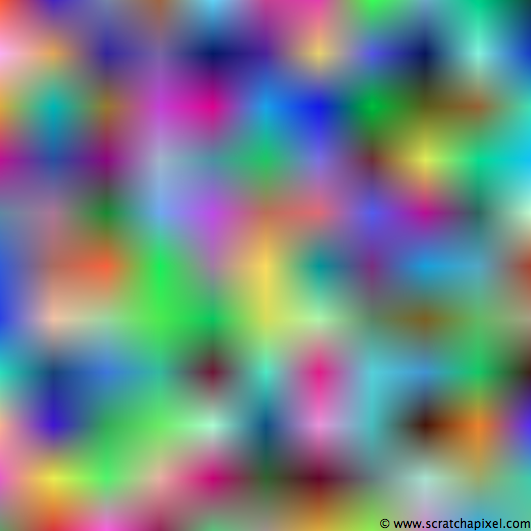
In the following example (complete source code is available for download), we create an image by interpolating the values (colors) of a grid for each pixel of that image. Many of the image pixels have coordinates that do not overlap the grid's coordinates. We use bilinear interpolation to compute interpolated colors at these "pixel" positions.

float bilinear(
   const float &tx, 
   const float &ty, 
   const Vec3f &c00, 
   const Vec3f &c10,
   const Vec3f &c01,
   const Vec3f &c11)
{
#if 1
    float a = c00 * (1 - tx) + c10 * tx;
    float b = c01 * (1 - tx) + c11 * tx;
    return a * (1 - ty) + b * ty;
#else
    return (1 - tx) * (1 - ty) * c00 + 
           tx * (1 - ty) * c10 +
           (1 - tx) * ty * c01 +
           tx * ty * c11;
#endif
}
 
void testBilinearInterpolation()
{
    // Testing bilinear interpolation
    int imageWidth = 512;
    int gridSizeX = 9, gridSizeY = 9;
    Vec3f *grid2d = new Vec3f[(gridSizeX + 1) * (gridSizeY + 1)]; // Lattices
    // Fill the grid with random colors
    for (int j = 0, k = 0; j <= gridSizeY; ++j) {
        for (int i = 0; i <= gridSizeX; ++i, ++k) {
            grid2d[j * (gridSizeX + 1) + i] = Vec3f(drand48(), drand48(), drand48());
        }
    }
    // Now compute our final image using bilinear interpolation
    Vec3f *imageData = new Vec3f[imageWidth * imageWidth], *pixel = imageData;
    for (int j = 0; j < imageWidth; ++j) {
        for (int i = 0; i < imageWidth; ++i) {
            // Convert i, j to grid coordinates
            float gx = i / float(imageWidth) * gridSizeX; // Be careful to interpolate boundaries
            float gy = j / float(imageWidth) * gridSizeY; // Be careful to interpolate boundaries
            int gxi = int(gx);
            int gyi = int(gy);
            const Vec3f &c00 = grid2d[gyi * (gridSizeX + 1) + gxi];
            const Vec3f &c10 = grid2d[gyi * (gridSizeX + 1) + (gxi + 1)];
            const Vec3f &c01 = grid2d[(gyi + 1) * (gridSizeX + 1) + gxi];
            const Vec3f &c11 = grid2d[(gyi + 1) * (gridSizeX + 1) + (gxi + 1)];
            *(pixel++) = bilinear(gx - gxi, gy - gyi, c00, c10, c01, c11);
        }
    }
    saveToPPM("./bilinear.ppm", imageData, imageWidth, imageWidth);
    delete [] imageData;    
}

The bilinear function is a template so you can interpolate data of any type (e.g., float, color). Notice also that the function can compute the same result in two different ways. The first method is more readable (#if 1 ...), but some people prefer to use the second method (#else ...) because the interpolation can be seen as a weighted sum of the four vertices. It's weighted because c00, c01, c10, and c11 are multiplied by some coefficients. For instance, (1 - tx) * (1 - ty) is the weighting coefficient for c00.

The advantage of bilinear interpolation is that it is fast and simple to implement. However, if you look at the second image in Figure 2, you will see that bilinear interpolation creates some patterns that may not be acceptable depending on what you intend to use the result of the interpolation for. If you need a better result, you will need to use more advanced interpolation techniques involving interpolation functions of degree two or higher (such as the smoothstep function, which is used for generating procedural noise as described in the lesson Procedural Patterns and Noise: Part 1).