Monte Carlo Simulation
Reading time: 44 mins.The content of this chapter is exclusive and copyrighted. Please do not copy and/or distribute without the permission of Scrathapixel. This free content requires hours of work and is totally unique on the web. If you found it useful, please consider making a donation.
Simulating Neutrons Transport
As mentioned in the introduction of this lesson, Monte Carlo methods were initially developed by scientists such as von Neumann, Metropolis, and Ulam who worked on atomic energy in the late 40s. One of their motivations (or one application they found of MC methods, one might never know if necessity here, was the mother of the invention), was to simulate the transport of neutrons through various materials. This is a long story; the maths and physics involved in this research are out of scope and won't be dealt with in this lesson. However, because this is probably the first and most interesting application of a Method Carlo method, we will present a version (an ersatz) of their experiment but quite simplified (not particularly accurate from a scientific point of view but still producing plausible results) and also without really explaining the origin of some of the equations involved. The same method can be used to simulate the propagation of light (photons) in tissue (skin) or smoke (for a complete introduction to light transport in participating medium, check the lessons on volume rendering and subsurface scattering in the advanced section).
Background
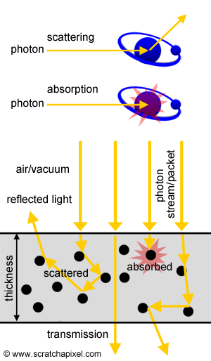
The program we will be using to explain the concept of MC simulation is based on equations and a mathematical framework that we won't explain in this lesson. The equations relate to the way light (photons) or neutrons propagates through tissues and other materials. Readers interested in this subject can find them explained in the lessons on sub-surface scattering and volume rendering. Don't stress out if you don't understand the maths used in this chapter (however most of the equations will be fully explained as usual). This is not the point of this chapter (and they are also explained in the lessons aforementioned). The point of this chapter is to show you the principle of a Monte Carlo simulation or the use of stochastic sampling to approximate the result of equations that are very hard or simply impossible to solve analytically. To understand the simulation though, you need to know a few basic things about the propagation of photons in tissues (the principles are the same for the interactions of neutrons with materials). This will eventually prepare you to read the lesson on volume rendering and subsurface scattering.
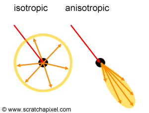
When a photon interacts with an object made of a certain material (we assume this object has a certain thickness), three things can happen to this photon as it travels through. If the photon interacts with an atom making up that material, it can either be absorbed (the energy of the photon is passed on to the atom which is returned back by the atom to its environment in the form of heat), or it can be scattered (the direction along which it travels is being changed). There's always the eventuality that the photon doesn't interact with an atom at all, in which case it just keeps traveling in the same direction until it eventually either interacts with an atom or leaves the object on the other side. The amount of light passing from one side of the object (or layer) to the other is called transmission. An illustration of these terms can be found in Figure 1. Note though that when a photon is scattered, its direction changes. If the photon is scattered in any random direction around the atom, we speak of isotropic scattering (the scattering is equal - iso means equal in greek - in all directions). However, sometimes, photons are being deflected within a given cone of directions centered around the photon's incoming direction. In this case, we speak of anisotropic scattering (the photon is not being scattered in all directions but within a preferred subset of directions centered about the photon's incoming traveling direction). In the case of anisotropic scattering, the new direction of a scattered photon can be computed using what we call a phase or angular function (check the lesson on subsurface or volume rendering to find more information on this function). In this chapter, we will only deal with isotropic scattering mostly to avoid complications in the code (we will thus assume that the photon can be scattered in any direction around the atom it interacts with). Check Figure 2 for a visual representation of these two scattering modes.
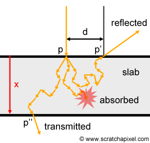
While bouncing from atom to atom, photons do follow some sort of random walk, which eventually leads some of them to leave the object on the side of the slab where they entered the object in the first place. Photons leaving the object on that side, make up what we call diffuse reflection or reflectance (the part of the light that is not being transmitted to the other side, but which is being reflected). In literature, it is often designated as Rd. However note that these photons enter and leave the object on the same side but not at the same point on the surface (they leave some distance away, noted \(d\) in Figure 3, from the point of illumination). In other words, light propagates. Which is the reason why "translucent" materials such as skin illuminated by a laser (or a collimated beam of light), do seem to scatter light away from the point of contact between the skin and the laser (Figure 3).

Photons escaping the slab on the other side though (the opposite side) contribute to what we call transmission (or transmittance), which is often denoted with the letter T (Figure 3).
In physics, two quantities can be used to define the property of a material to absorb and scatter photons. They are simply called, the absorption and scattering coefficients. They are usually denoted by the greek letter \(\sigma\) (sigma): \(\sigma_a\) for the absorption coefficient and \(\sigma_s\) for the scattering coefficients. They measure, the likelihood of a photon to be absorbed or scattered per unit length of material (the unit length can be millimeter, centimeter, etc.). In other words, the absorption coefficient, for instance, indicates how likely a photon is to be absorbed as it travels through a slab of material. Note that these values can be greater than 1\. They are not to be confused with probabilities even though the concept is very similar (remember that a probability can never be greater than 1). In physics, the rate at which the photon is being absorbed or scattered as it travels through a slab of material is defined by a very famous law named the Beer-Lambert law. The equation for this law can take on different forms. In this lesson we will use the following formula:
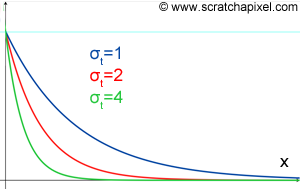
$$ \begin{array}{l} T & = & e^{-(\sigma_a + \sigma_s)x},\\ & = & e^{-\sigma_t x}. \end{array} $$where, \(\sigma_t = \sigma_a + \sigma_s\). This term \(\sigma_t\) (read "sigma t") is called the extinction coefficient. You can see a plot of this equation in Figure 4. If you are not familiar with the exponential function (the \(e\) term), we recommend you to plot the curve for different values of the \(\sigma_t\) (you can use Grapher on Mac or GnuPlot of Linux). The parameter \(x\), is the distance that the photon travels in the slab. This equation can be seen as the number of photons (or light) transmitted on the other side of the slab (which is why we use the term T in the equation above). As you can see by just looking at the graph, the greater the distance, the smaller the transmission, and the rate at which transmission decreases with distance, follows an exponential decay. The reason why transmission decreases with distance is that photons get absorbed along the way. So of course, the greater the distance they have to travel to escape the surface on the other side, the more likely they are to be absorbed.
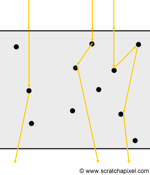
If we call \(x_i\) the distance from the point of incidence and the point in the slab where the \(i\) the photon is either scattered or absorbed, you can see by looking at Figure 5 that because each photon has its own "fate", this distance varies from photon to photon: some photons are scattered a short distance away from the point where they entered the slab, while some others travel a much larger distance before interacting with an atom. In fact, this distance which is known as the free path length, is ..., random. It should not come as a surprise to see this concept coming up again, since you should have realized by now, that the concept of a random variable is central to this lesson and the concept of Monte Carlo methods. The probability that a photon will be absorbed or scattered (as a function of distance) can be computed with the following equation:
$$p(x) = \sigma_t e^{-\sigma_t x}, \: 0 \lt x \lt \infty.$$Again, it is an exponential function and we know what this function looks like (Figure 4). It doesn't matter if you don't understand where these equations come from. You will find them explained in the lesson on subsurface scattering.
However, you should already be familiar though with the concept of probability and probability density function which we already talked about in the lesson Mathematical Foundations of Monte Carlo Methods) (in probability theory, a probability density function or pdf, is a function that describes the relative likelihood for this random variable to take on a given value). The equation above is an example of such pdf.
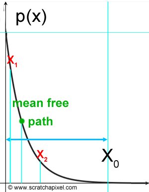
There is something interesting to note about this function: the probability decreases (it actually converges to 0) as the distance \(x\) increases. It might seem counter-intuitive at first because you could expect this probability to actually increase with \(x\) instead. Indeed, if the photon is not scattered or absorbed after some distance x, then we are almost sure that it will eventually be scattered or absorbed at some point further down along its path if it keeps traveling through the slab. Thus naturally, you might be inclined to think that the probability increases with distance. But in reality, the opposite is true. Why? If the probability of a photon to be scattered or absorbed converges to 0 for values of \(x\) greater than \(x_0\), the equation just tells us that the photon is more likely to be scattered or absorbed for a distance smaller than \(x_0\). For instance, if you look at Figure 6, the probability of a photon experiencing a scattering event is greater at distance \(x_1\) than it is at distance \(x_2\). In other words, you are almost certain that the photon is more likely to be scattered or absorbed for distances smaller than \(x_0\) thus the probability itself for a photon to be scattered for a distance greater than \(x_0\) becomes very small. It is an important point to understand and remember.
Finally, let's mention that the probability of a photon being absorbed is \(\sigma_a / \sigma_t\) and its probability to be scattered is \(\sigma_s / \sigma_t\).
Principle of the Experiment: Let's Simulate!
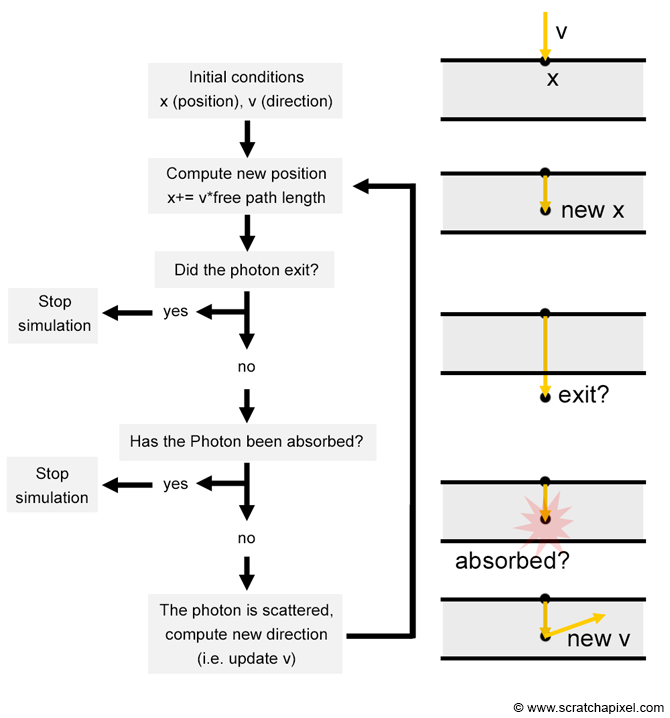
What if we could use a computer to simulate the path of a photon traveling through a slab of material? The idea is pretty simple. All we need to do is create a virtual photon, initially place it at the surface of the slab and simulate its random walk which can be done by executing the following decision tree:
-
Step 1: compute the new position of the photon. Move along some distance away from the current position \(x\) in the direction \(v\).
-
Step 2: is the photon still traveling through the slab? This can be easily tested by computing the position of the photon and comparing it to the boundaries of the slab.
-
If the photon is outside the slab boundaries, stop the simulation.
-
If the photon is still traveling through the slab, continue.
-
-
Step 3: at this stage, the photon can either be absorbed or scattered. Compute the photon probability to either be absorbed or scattered (using the absorption and scattering coefficient).
-
If the photon is absorbed, stop the simulation (the photon disappeared)
-
If the photon is scattered, update the direction along which the photon travels (\(v\)) and go back to step 1.
-
Here is a visual representation of that tree:
If we repeat this experiment thousands of times, eventually, in the end, we get an estimation of how much light is reflected or transmitted by this slab of material. The main difficulty with the process described above though is to determine the distance by which we should be moving the photon over, at each iteration of the loop. Technically, this distance which we know is called the free path length, should be chosen randomly however what should it be? Short, long, one time short, the next time long? Surely, the choice of distance, however random, must be related somehow to the properties of the material themselves, notably its scattering and absorption coefficient (which we talked about already). Indeed, we can guess that if the absorption and the scattering coefficients for example are very low, then the likelihood of a photon being absorbed or reflected is also low. Thus distances between scattering events should be long in that case. Of course, the opposite is true. When these coefficients have high values, the probability of a photon interacting with an atom is high, so you should expect distances between scattering events to be short. This likelihood is actually defined by the equation for the PDF we introduced earlier on;
$$P(x) = \sigma_t e^{-\sigma_t x}.$$This says that the probability that the photon interacts with an atom decreases exponentially with the distance x (where "how quickly this probability decreases is controlled by the extinction coefficient which is the sum of the absorption and scattering coefficient). What we need for our exercise, is to generate x's (random distances at which the photon will be scattered or absorbed), but with the same probability density function as this PDF. If you look at Figure 6 again, there's a higher probability for x to have values around the mean free path than values approaching infinity, thus if you sample x (i.e., generate random values for x), you should also get more x's with values around the mean free path than values approaching infinity. This is what "sampling a random number based on a given PDF" means.
In the lesson Mathematical Foundations of Monte Carlo Methods, we learned how to sample a random variable X using any given distribution. The method we described is called the Inverse Transform Sampling method. First, we need to build a CDF from the PDF. In our case, this CDF defines the probability for a photon to interact with an atom within any distance lower than a certain given value x:
$$CDF(x) = Pr(\text{ Interaction Distance } < x).$$Remember that a probability can only take on a value within the range [0,1]. The idea behind the inverse sampling method is to somehow invert the CDF so that the output of the CDF (the probability) becomes the input of the inverted CDF, and the input of the CDF (the distance x at which the photon is scattered) becomes the output of the inverted CDF:
$$invCDF(\xi) = x.$$By feeding this inverted CDF with random numbers uniformly distributed, we can generate values for x with the desired PDF (this method is described in detail in lesson 16). We also learned in lesson 16, that for some PDFs, the CDF can be computed analytically, which luckily enough, is the case for the exponential distribution function. The inverted CDF of the PDF:
\(PDF(x) = a e^{-a x}\) is \(x = - \dfrac{\ln(\xi)}{a}\).
The derivation for this formula can be found in the lesson Mathematical Foundations of Monte Carlo Methods. In our case \(a\) is equal to \(\sigma_t\), the extinction coefficient.
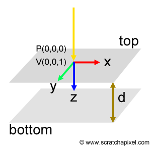
Where is that taking us? Now that we have a method for sampling x, we have all we need to write the code of our MC simulation. The conditions of our experiment will be the following. We will have a slab of material whose thickness d is known. What we also know about this material is its absorption and scattering coefficient. For all our experiments, we will assume a Cartesian coordinate system in which the z-axis points downwards and the xy plane lies within the top surface of the slab (Figure 7). The position and direction of the photon traveling through the material sample will be defined in this coordinate system. What's the goal of this simulation? The goal is to follow the path of a photon as it travels through the slab. Initially, we will assume that the direction of this photon is perpendicular to the slab's top surface. In other words, its original direction is (0,0,1). Next, we will enter an infinite loop from which we will not go away until the photon potentially leaves the slab or until it gets absorbed.
Vec3f P(0,0,0);  //orignal position of the photon in our simulation
Vec3f V(0,0,1);  //original direction
while (1) {
   if (photon leaves surface) break;
   if (photon is absorbed) break;
}
However, following the path of one photon is not really interesting. What we want indeed, is to know how many photons on average are either reflected through the top surface (diffuse reflectance), transmitted through the bottom surface, or absorbed. To make this simulation useful, we will actually run the same inner loop for a great number of photons and count which ones are absorbed, reflected, or transmitted.
int photon = 10000;
int Rd = 0;  //diffuse reflectance, number of photons leaving the slab through the top surface
int Tt = 0;  //number of photons leaving the slab through the bottom surface
int A = 0;  //number of absorbed photons
for (int i = 0; i < nphotons; ++i) {
    Vec3f P(0,0,0);  //orignal position of the photon in our simulation
    Vec3f V(0,0,1);  //original direction
    while (1) {
        if (photon leaves surface) {
            if (photon leaves through top surface) Rd++;  //diffuse reflectance
            else Tt++;  //transmittance
            break;
        }
        ...
        if (photon is absorbed) { A++; break; }
    }
}
printf("Rd %f Tt %f Absorption %f\n", Rd / nphotons, Tt / nphotons, A / nphotons;
Because the distance x at which the photon is scattered and the new direction it follows while being scattered is different for each photon and each scattering event, each photon has a unique path. But on average, as the number of photons approaches a very large number, diffuse reflectance, transmittance, and absorption will converge. This is the principle and the goal of this Monte Carlo simulation. Getting an estimation or approximation for these values by simulating a great number of photon paths and averaging the results. The greater the number of photons, the more accurate this approximation is likely to be, however, of course, the simulation time also increases with this number.
The first thing we will do, at each new iteration of this loop, computes some distance x using the inverted CDF of the exponential distribution.
$$x = - \dfrac{\ln(\xi )}{\sigma_t },$$where \(\epsilon\) is a random number uniformly distributed in the range [0,1]. In C/C++, we can use a call drand48() for this or a more sophisticated solution if you use C++11.
float x = -ln(drand48())/sigma_t; //where sigma_t = sigma_a + sigma_s
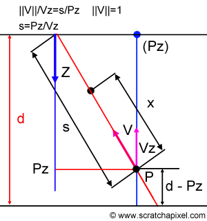
Next, we will move the photon to its new position, using its direction and the sampled value for x. However, before we do this, we need to check that while moving the photon we won't be leaving the slab. This can easily be done by computing the distance from the actual position of the photon to the top and bottom surface of the slab and comparing this distance with the sampled distance x. If x is greater than this distance, the photon will actually go across the boundaries of the slab and leave it. Computing this distance is a simple geometric problem. As you can see in Figure 8, we want to find the distance s. Using the technique of similar triangles which says that the corresponding sides of two similar triangles have the same ratio. Thus we can write that:
$${||V|| \over V_z} = \dfrac{s}{P_z}.$$Since V is a normalized vector its length is equal to 1. From there we find for s:
$$s = \dfrac{P_z}{V_z}.$$We still have to check whether V is pointing towards the top or the bottom surface. If it points to the bottom surface (which is true if \(V_z\) is greater than 0), the equation for s is slightly different:
$$s = \dfrac{(d - P_z)}{V_z}.$$
float s = (V.z > 0) ? (d - P.z) / V.z : - P.z / V.z;
if (x > s) {  //yes we leave the slab
    if (P.z > 0) Rd++;  //contribution to diffuse reflectance
    else Tt++;  //contribution to transmittance
    break;  //we can stop following the path of the photon so let's break
}
If the photon leaves the slab through the top surface, it will contribute to diffuse reflectance. We can track this by incrementing a variable which is used to count the number of photons leaving the slab through the top surface (diffuse reflectance). If it leaves the slab through the bottom surface instead, we can do the same but this time increment a variable that is used to track the number of photons leaving the slab through the bottom surface (transmittance). Finally, if the photon leaves the slab, there's no point continuing following its path. So we can break from the loop.
If the photon doesn't leave the slab on its next move, we can update its position.
// P and V are the position and direction of the photon respectively
P.x = P.x + x * V.x;
P.y = P.y + y * V.y;
P.z = P.z + z * V.z;
The next position of the photon corresponds to an interaction between the photon and an atom in the slab. Thus, we want to check if, during this scattering event, the photon is being absorbed or scattered. If the photon is absorbed, it "dies". We can then update the counter keeping track of the number of photons absorbed, break the loop and move on to the next photon. The way we check if the photon is absorbed or not is by simply comparing whether some random variable uniformly distributed is lower than the probability of a photon to be absorbed which is \(\sigma_a / \sigma_t\).
if (drand48() < sigma_a / sigma_t) {
    absorption++;
    break;
}
However, most MC simulations use a different approach to solve this problem. In fact, simulating photons one by one is quite tedious. What we can do instead is consider that we actually follow a packet of photons, which are following the same path instead. As these photons travel through the medium, some of them are absorbed. The way we keep track of how much of the photons have been absorbed is by assigning a weight to the packet of photons. This weight is initially set to 1\. The probability that a photon gets absorbed (\(\sigma_a / \sigma_t\)) can also be seen as the portion (in percentage if you prefer to see it that way) that say 100 photons for instance get absorbed while interacting with an atom. Thus at each scattering event, what we will do is decrease the weight of the packet by this ratio.
int photons = 10000;
...
float absorption = 0;
for (int i = 0; i < nphotons; ++i) {
    float w = 1;  //set the weight to 1
    Vec3f P(0, 0, 0);
    Vec3f V(0, 0, 1);
    while (1) {
        ...
        float dw = sigma_a / sigma_t;
        absorption += dw;
        w -= dw;
        if (w <= 0) {
            break;
        }
    }
}
As you can see with the code though, we changed the way we now compute the absorption. Because we don't count individual photons anymore, we will keep track instead of the portion of photons that are being absorbed from the packet. We can break out of the loop when the weight is lower or equal to 0. However, here again, it is common to use a technique called Russian roulette. What this technique does from a mathematical point of view will be explained in the lesson on Light Transport. However, the idea is that when the weight of the packet becomes really small (you can set the threshold yourself) we can stochastically decide to either kill the packet altogether or let it travel through the slab. However, because this test modifies the "fate" of the packet, if the packet passes the test, we will need to adjust its weight accordingly. You often use the Russian roulette technique when it comes to using Monte Carlo methods for evaluating/approximating integrals (see for example the lesson on Volume Rendering and Ray Marching).
int photons = 10000;
...
int m = 5;  //there's 1 over 6 chances for the packet to be absorbed
for (int i = 0; i < nphotons; ++i) {
    float w = 1;  //set the weight to 1
    Vec3f P(0, 0, 0);
    Vec3f V(0, 0, 1);
    while (1) {
        ...
        float dw = sigma_a / sigma_t;
        absorption += dw;
        w -= dw;
        if (w < 0.001) {  //perform russian roulette if weight is small
            if (drand48() < 1.0 / m) {
                break;  //we kill the packet
            }
            else
                w *= m;  //adjust weight
        }
    }
}
As you can see with this code, the fate of the packet is decided by the variable \(m\). You can see it as the number of bullets a gun can hold in its barrel. If you assume that only one of the chambers in the gun is loaded, then what the test does is find out whether you get killed by the bullet or not. If \(m\) is the total number of chambers in the gun's cylinder, the probability of the packet getting killed is 1 over m. If you don't understand why the weight of the packet is multiplied by \(m\), if it survives the test, we recommend that you read the lesson on Light Transport. However, as a quick explanation, you can think of it this way: Russian roulette will have the effect of "prematurely" killing some of the packets. In effect, this introduces some bias because using Russian roulette changes the fate of the packets and thus the potential results of the simulation (compared to the unbiased version which is the version that doesn't use a Russian roulette test). Thus we need to account for the "prematurely" disappearance" of these packets, by providing the packets that survived a longer lifespan (which you can do by multiplying the weight by m). In other words, we compensate for the packets which have been prematurely killed by increasing the lifespan of the surviving ones, proportionally to the chance that a packet gets killed. This process keeps the simulation unbiased.
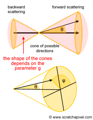
Finally, if the photon or the packet of photons doesn't get killed, it is instead scattered. From a code point of view, it means that we need to compute a new direction for this packet (update the vector V). This part of the code is never the simplest because as we mentioned earlier in the introduction of this chapter, the material making up the slab can either be isotropic (photons will then be scattered in all possible directions) or anisotropic (photons are " mostly" scattered within a cone of directions centered around the photon traveling direction). The new direction can be computed by sampling what is called a phase function. One of the most popular phase functions in computer graphics is called the Henyey-Greenstein scattering phase function. You can find a detailed explanation of this topic in the lesson on Volume Rendering. This function only takes one parameter usually denoted g. When g is equal to 1, photons are scattered in the same direction as the photon's incoming direction. A value of 0 means the medium is isotropic. Values in the middle mean, that photons are mostly scattered within a cone of directions centered around the photon traveling direction (see Figures 2 and 9). In fact, the phase function says that photons can also be scattered in a cone of directions centered along the photon opposite incoming direction. So photons are actually scattered forward and backward but the amount of forward scattering vs. backward scattering depends on the parameter g. When g is greater than 0, forward scattering is dominant, while for g lower than 0, backward scattering dominates (see Figure 9). The scattering function returns the cosine of the angle \(\theta\) which is the deflection angle (see Figure 9). To sample the Henyey-Greenstein function we will use the following formula (see the note below for a derivation of the formula):
$$ \begin{cases} \dfrac{1}{2g} \left[ 1 + g^2 - \left(\dfrac{1-g^2}{1-g+2g\xi}\right)^2\right]&\text{ if }g\ne 0 \\ 1-2\xi&\text{ if }g= 0 \end{cases}, $$where as usual, \(\xi\) is a random number in the range [0,1] uniformly distributed.
The Henyey-Greenstein scattering phase function is a probability density function. It returns the probability of a photon to be scattered for a given deflection angle \(\theta\). The formula for the function is:
$$p(\theta) = \dfrac{1}{4 \pi} \dfrac{1 - g^2}{(1 + g^2 - 2g \cos(\theta))^{3/2}}.$$As with every PDF, the integral of this function is unity. You will need to integrate over \(4\pi\) radians:
$$\int_0^{2\pi} \left\{ \int_0^\pi p(\theta) sin(\theta) d \theta \right\} d \phi = 1.$$You can find a derivation of this result in the lesson on Volume Rendering. We know from the lesson Mathematical Foundations of Monte Carlo Methods, that to sample a PDF, we need to compute its CDF and invert it. We can write the H-G function in a simpler way by substituting the greek letter \(\mu\) to \(\cos(\theta)\):
$$p(\mu) = \dfrac{1}{2} \dfrac{1 - g^2}{(1 + g^2 - 2g \mu)^{3/2}},$$and then:
$$\int_{-1}^1 p(\mu) d\mu = 1.$$Check the result of the function \(p(\mu)\) for some values of \(\mu\). For example when \(\scriptsize\mu = -1\) (or when \(\theta = 0\)) and \(\mu = 1\) (\(\theta = \pi\)).
Remember that the CDF of a PDF returns the probability that a random variable X takes on any value lower than some possible outcome. Keep in mind the example of dice: the CDF(Pr < 4) returns the probability that a throw of dice returns any value lower or equal to 4 (which is 4/6 in the case of a dice). The CDF of our H-G needs to return the probability for any angle to be lower or equal to say \(\mu'\).
$$\text{CDF}(\text{ Pr } < \mu') = \dfrac{1}{2} \int_{-1}^{\mu'} {\dfrac{(1 - g^2)d\mu}{(1 + g^2 - 2g \mu)^{3/2}}}.$$To find a solution to this problem, we need to integrate over the domain [-1,\(\mu'\)], and to do so, we will use the second fundamental theorem of calculus which we introduced in the chapter The Mathematics of Shading [link]. As a quick reminder:
$$\int_a^b f(x) dx = F(b) - F(a),$$where F(x) is the antiderivative of f(x). What we need to do now is to find the antiderivative of the function to the right of the integral sign. To understand the derivation, remember that according to the power rule the derivative of \(x^n\) is \(nx^{n-1}\) and also that the derivative of \((c + 2ax)^n\) is \(2an(c + 2ax)^{n-1}\) (obviously the number 2 here can be any other value and c is a constant and be careful with the sign in front of 2ax, it can be negative which is the case in our function). Remember too that any expression such as:
$$\dfrac{1}{x^{1/2}}$$can be written as \(x^{-1/2}.\) With this in hand we can re-write:
$$\dfrac{1}{ (1 + g^2 - 2g \mu )^{3/2}},$$as:
$$(1 + g^2 - 2g\mu)^{-3/2}.$$To find the anti-derivative, of this function we will use the power rule. If the exponent of the derivative function is 3/2, according to the power rule, it was calculated as n - 1 = -3/2 thus the exponent of the antiderivative is n = -3/2 + 1 = -1/2. If for instance we want to find the derivative of \((1+g^2-2gx)^{-1/2}\), then we would find:
$$(-2g)( -\dfrac{1}{2}) (1 + g^2 - 2gx)^{-3/2},$$thus if the final derivative is \((1 + g^2 - 2gx)^{-3/2}\), our antiderivative has to be:
$$\dfrac{1}{g }(1 + g^2 - 2g \mu)^{-1/2}.$$If we now move this result back to the denominator we have:
$$\dfrac{1}{{g (1 + g^2 - 2g \mu)}^{1/2}}.$$Our final antiderivative function is:
$$\dfrac{1}{2} {\dfrac{1 - g^2 }{g \sqrt{1 + g^2 - 2g \mu}}}.$$We can now integrate using the second fundamental theorem of calculus:
$$ \begin{array}{l} CDF(\mu') & = & \left [ {1 \over 2} {\dfrac{1 - g^2 }{g \sqrt{1 + g^2 - 2g \mu}} } \right]_{-1}^{\mu'}\\ & = & \dfrac{1}{2} {\dfrac{1 - g^2 }{g \sqrt{1 + g^2 - 2g \mu'}} } - \dfrac{1}{2} {\dfrac{1 - g^2 }{g \sqrt{1 + g^2 + 2g}} }\\ & = & \dfrac{(1 - g^2)}{2g}( {\dfrac{1}{\sqrt{1 + g^2 - 2g \mu'}} } - {\dfrac{1}{{1 + g}} }). \end{array} $$And invert the CDF to express \(\mu\) as a function of the probability. If we write:
$$\xi = \dfrac{(1 - g^2)}{2g} ( {\dfrac{1}{\sqrt{1 + g^2 - 2g \mu'} } } - {\dfrac{1}{{1 + g}}}).$$Derivation:
$${\dfrac{2g \xi }{ 1 - g^2 } } = \dfrac{1}{\sqrt{(1 + g^2 - 2g \mu}} - \dfrac{1}{1 + g}$$ $${ 1 \over {\sqrt{1 + g^2 - 2g \mu} } } = {{2 g \xi} \over {1 - g^2}} + { 1 \over { 1 + g }}$$ $${ 1 \over {\sqrt{1 + g^2 - 2g \mu} } } = {{2 g \xi} \over {1 - g^2}} + { (1 - g) \over {( 1 + g)(1 -g) }}$$ $${ 1 \over {\sqrt{1 + g^2 - 2g \mu} } } = { {2 g \xi} \over {1 - g^2} } + { ( 1 - g) \over { (1 - g)^2 } }$$ $${ 1 \over {\sqrt{1 + g^2 - 2g \mu} } } = {{2 g \xi + (1 - g)} \over {1 - g^2}} $$ $${ {\sqrt{1 + g^2 - 2g \mu} } } = { {1 - g^2} \over {2 g \xi + (1 - g)} } $$ $${ {{1 + g^2 - 2g \mu} } } = \left( { {1 - g^2} \over {2 g \xi + (1 - g)} } \right)^2 $$ $$ \mu = {{1} \over { 2g}} \left( 1 + g^2 -\left( { {1 - g^2} \over {2 g \xi + (1 - g)} } \right)^2\right).$$And we get:
$$\mu = \frac{1}{2g} \left[ 1 + g^2 - \left(\frac{1-g^2}{1-g+2g\xi}\right)^2\right],$$which is the function we will be using to sample \(\cos(\theta)\).
Now that we know how to sample the deflecting angle (\(\cos\theta\)), what we need is some formula to rotate the photon incident direction. Remember that the photon needs to rotate both in \(\theta\) and \(\phi\) (see Figure 9). The formulas for each coordinate of the new direction vector are as follows:
$$ \begin{align} \mu'_x & = \mu_x \cos\theta + \frac{\sin\theta(\mu_x \mu_z \cos\phi - \mu_y \sin\phi)}{\sqrt{1-\mu_z^2}}\\ \mu'_y & = \mu_y \cos\theta + \frac{\sin\theta(\mu_y \mu_z \cos\phi + \mu_x \sin\phi)}{\sqrt{1-\mu_z^2}} \\ \mu'_z & = \mu_z \cos\theta - \sqrt{1-\mu_z^2}\sin\theta\cos\phi \\ \end{align} $$Where these formulas come from is explained in the note box below.
One common method for rotating a vector v around another k is called Rodrigues' rotation formula. This method is explained in detail in the advanced section of the lesson on Geometry (lesson 4). As a reminder, the formula is as follow:
$$v_{rot} = \cos(\theta) v + \sin(\theta) (k \times v) - k (k . v) (1 - \cos(\theta)).$$In our case, and we will show this in a moment, we will construct a vector k orthogonal to v. Thus if \((k.v) = 0\) the formula reduces to \(v_{rot} = \cos(\theta) v + \sin(\theta) (k \times v)\). The question now is "how do we find k".
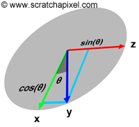
Start with unit vector \(\mathbf{\hat{x}}\equiv(u_o, v_o, w_o)\). We wish to compute all unit vectors \(\mathbf{\hat{y}}\) such that the angle between \(\mathbf{\hat{x}}\) and \(\mathbf{\hat{y}}\) is \(\theta \), i.e., \(\mathbf{\hat{x}}\cdot\mathbf{\hat{y}}=\cos\theta \).
It is easy to see that \(\mathbf{\hat{y}}\) is a unit vector such that \(\mathbf{\hat{x}}\cdot\mathbf{\hat{y}}=\cos\theta\) if and only if
$$\mathbf{\hat{y}} = \cos\theta \mathbf{\hat{x}} + \sin\theta \mathbf{\hat{z}}$$for some unit vector \(\mathbf{\hat{z}}\) orthogonal to \(\mathbf{\hat{x}}\). (Proof: Suppose \(\mathbf{\hat{y}} = \cos\theta \mathbf{\hat{x}} + \sin\theta \mathbf{\hat{z}}\) where \(\mathbf{\hat{x}}\cdot\mathbf{\hat{z}}=0\). Then \(\mathbf{\hat{x}}\cdot\mathbf{\hat{y}}=\cos\theta\). Conversely, suppose \(\mathbf{\hat{y}}\) is a unit vector with \(\mathbf{\hat{x}}\cdot\mathbf{\hat{y}}=\cos\theta\). Then
$$\mathbf{\hat{y}} = \cos\theta\mathbf{\hat{x}} + \frac{\mathbf{\hat{y}}-\cos\theta\mathbf{\hat{x}}}{\| \mathbf{\hat{y}}-\cos\theta\mathbf{\hat{x}}\|}\| \mathbf{\hat{y}}-\cos\theta\mathbf{\hat{x}}\|.$$But, \(\|\mathbf{\hat{y}} - \cos\theta\mathbf{\hat{x}}\| = \sqrt{(\mathbf{\hat{y}} - \cos\theta\mathbf{\hat{x}})\cdot(\mathbf{\hat{y}} - \cos\theta\mathbf{\hat{x}})} = \sqrt{1-2\cos\theta + \cos^2\theta} = \sin\theta\)
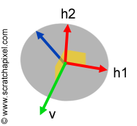
Next, we characterize all unit vectors orthogonal to \(\mathbf{\hat{x}}\). Since we are in \(\mathbb{R}^3\), the set of vectors orthogonal to \(\mathbf{\hat{x}}\) is a 2-dimensional dimensional vector space (the grey disk in the adjacent image). If we find two unit vectors \(\mathbf{\hat{h}_1}\) and \(\mathbf{\hat{h}_2}\) that are orthogonal to one another and to \(\mathbf{\hat{x}}\), then every unit vector orthogonal to \(\mathbf{\hat{x}}\) can be written as
$$\alpha \mathbf{\hat{h}_1} + \beta \mathbf{\hat{h}_2}$$for some \(\alpha\), \(\beta\) where \(\alpha^2+\beta^2=1\). (The proof is easy.)
Here are two vectors orthogonal to \(\mathbf{\hat{x}}\equiv(u_o,v_o,w_o)\) and to each other:
$$ \begin{array}{l} (-v_o,u_o,0) \\ (u_o w_o, v_o w_o, -u_o^2 - v_o^2). \end{array} $$Lots of other vectors could have been chosen. We found the first of these two vectors by examining the formulas provided. We computed the second as the vector cross product of \(\mathbf{\hat{x}}\) and the first vector. This ensures mutual orthogonality. Each of these two vectors has length \(\sqrt{u_o^2 + v_o^2} = \sqrt{1-w_o^2}\). We can normalize each to obtain:
$$ \begin{array}{l} \mathbf{\hat{h}_1} &=& \frac{1}{\sqrt{1-w_o^2}}(-v_o,u_o,0) \\ \mathbf{\hat{h}_2} &=& \frac{1}{\sqrt{1-w_o^2}}(u_o w_o, v_o w_o, -(1- w_o^2)). \end{array} $$Putting all this together, we can compute \(\mathbf{\hat{y}}\) as
$$ \begin{array}{l} \mathbf{\hat{y}}\equiv(u,v,w) &=& \cos\theta\ \ (u_o,v_o,w_o) + \alpha\sin\theta\frac{1}{\sqrt{1-w_o^2}}(-v_o,u_o,0) \\ & & + \beta\sin\theta\ \ \frac{1}{\sqrt{1-w_o^2}}(u_o w_o, v_o w_o, -(1-w_o^2)). \end{array} $$Now just set:
$$ \begin{array}{l} \alpha & = & \frac{\xi_2}{\sqrt{\xi_1^2 + \xi_2^2}} \\ \beta & = & \frac{\xi_1}{\sqrt{\xi_1^2 + \xi_2^2}} \\ \cos\theta & =& \mu_{lab} \\ \sin\theta & = & \sqrt{1-\mu_{lab}^2} \end{array} $$and we have the formulas we started with.
Once the new direction of the photon is computed, we start from the top of the loop again and repeat this process until the photons get absorbed or leave the slab. Once the path of all the photons is simulated, we will need to normalize the Rd and Tt variables by dividing their value by the total number of photons. This will give us a percentage of light that was transmitted vs reflected. The total of these two numbers is not necessarily equal to 1, as a fraction of the photons may have been absorbed before leaving the slab. Finally, here is a C++ implementation of the entire photon transport algorithm (the complete source is available from the download section of this lesson):
double getCosTheta(const double &g) // sampling the H-G scattering phase function
{
    if (g == 0) return 2 * drand48() - 1;
    double mu = (1 - g * g) / (1 - g + 2 * g * drand48());
    return (1 + g * g - mu * mu) / (2.0 * g);
}

void spin(double &mu_x, double &mu_y, double &mu_z, const double &g)
{
    double costheta = getCosTheta(g);
    double phi = 2 * M_PI * drand48();
    double sintheta = sqrt(1.0 - costheta * costheta); // sin(theta)
    double sinphi = sin(phi);
    double cosphi = cos(phi);
    if (mu_z == 1.0) {
        mu_x = sintheta * cosphi;
        mu_y = sintheta * sinphi;
        mu_z = costheta;
    }
    else if (mu_z == -1.0) {
        mu_x = sintheta * cosphi;
        mu_y = -sintheta * sinphi;
        mu_z = -costheta;
    }
    else {
        double denom = sqrt(1.0 - mu_z * mu_z);
        double muzcosphi = mu_z * cosphi;
        double ux = sintheta * (mu_x * muzcosphi - mu_y * sinphi) / denom + mu_x * costheta;
        double uy = sintheta * (mu_y * muzcosphi + mu_x * sinphi) / denom + mu_y * costheta;
        double uz = -denom * sintheta * cosphi + mu_z * costheta;
        mu_x = ux, mu_y = uy, mu_z = uz;
    }
}

void MCSimulation()
{
    // compute diffuse reflectance and transmittance
    uint32_t nphotons = 100000;
    double scale = 1.0 / nphotons;
    double sigma_a = 1, sigma_s = 2, sigma_t = sigma_a + sigma_s;
    double d = 0.1, g = 0.75;
    static const short m = 10;
    double Rd = 0, Tt = 0;
    for (int n = 0; n < nphotons; ++n) {
        double w = 1;
        double x = 0, y = 0, z = 0, mux = 0, muy = 0, muz = 1;
        while (1) {
            double s = -log(drand48()) / sigma_t;
            double distToBoundary = 0;
            if (muz > 0) distToBoundary = (d - z) / muz;
            else if (muz < 0) distToBoundary = -z / muz;
            if (s > distToBoundary) {
                if (muz > 0) Tt += w; else Rd += w;
                break;
            }
            // move
            x += s * mux;
            y += s * muy;
            z += s * muz;
            // absorb
            double dw = sigma_a / sigma_t;
            w -= dw; w = std::min(0.0, w);
            if (w < 0.001) { // russian roulette test
                if (drand48() > 1.0 / m) break;
                else w *= m;
            }
            // scatter
            spin(mux, muy, muz, g);
        }
    }
    printf("Rd %f Tt %f\n", Rd * scale, Tt * scale);
}
However functional, this code is not great for people who are more interested in visual results. One of the things we can do is visualize the result of the transmission. The idea is to create a 2D array or a 2D grid of bins representing the bottom surface of the slab. If a photon leaves the slab through the bottom surface, we will compute its grid position (from the photon's xy coordinates), and add the photon's weight to the bin it falls into (see diagram below - right). At the end of the simulation, the content of the grid can be saved as an image and displayed (below - left).
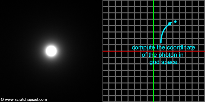
As you can see with the result of this photon transport simulation, the diffusion of photons (or the distribution of these photons due to scattering) around the incident beam is perfectly symmetrical. While eventually hard to see with this example, the falloff from the center of the diffusion halo to the edge of the halo follows an exponential decay. The pseudo-code for storing the photon's weight looks like this (check the source code in the download section of this lesson):
float *records = NULL;
int weight = 512, height = 512;
records = new float[width * height];
memset(record, 0x0, sizeof(float) * width * height);
void MCSimulation()
{
    // just deposit photon on the surface of the slab
    uint32_t nphotons = 100000;
    double scale = 1.0 / nphotons;
    double sigma_a = 1, sigma_s = 2, sigma_t = sigma_a + sigma_s;
    double d = 0.1, slabwidth = 5, g = 0.75;
    static const short m = 10;
    uint32_t Rd = 0, Tt = 0;
    for (int n = 0; n < nphotons; ++n) {
        ...
        while (1) {
            ...
            if (s > distToBoundary) {
                int xi = (int)((x + slabwidth / 2) / slabwidth * width);
                int yi = (int)((y + slabwidth / 2) / slabwidth * width);
                if (muz > 0 && xi >= 0 && x < width && yi >= 0 && yi < height) {
                    records[yi * width + xi] += w;
                }
                break;
            }
            ...
        }
    }
    // normalize
    for (int i = 0; i < width * height * 3; ++i) record[i] *= scale;
}
Depending on your absorption and scattering coefficients you may have to scale the values stored in the bins of the grid up or down to actually see something. Besides playing with scattering coefficients, you can also change the thickness (d) of the slab and look at the different results you get. The higher the absorption and scattering coefficient, the less translucent the material (gif animation below, left). As you increase the thickness of the slab, you can see how light from the beam becomes more and more diffuse (gif animation below, right)
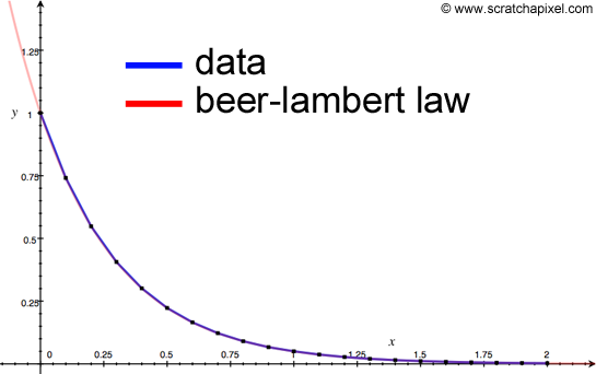
To double-check that out experiment (and approach) is working we can compute transmission for increasing values of d (the thickness of the slab) and compare the result to the equation of the Beer-Lambert Law (\(T = e^{-\sigma_t x}\)). The changes to the code are easy:
void MCSimulation(double d) // where d is the depth of the slab
{
    ....
}

for (int i = 0; i <= 20; ++i) {
    MCSimulation(i / 20. * 2); // 21 steps over a slab with thickness 2
}
Our simulation gives results that are really close to the prediction. The two curves (the experiment curves in blue and a plot of the Beer-Lambert Law in red) match almost perfectly (you need to set g to 0):
This concludes our work on implementing a photon transport algorithm using Monte Carlo. As you can see the technique gives very good results, close to the predictions. It shows you the power of this method as well as its simplicity. Monte Carlo in this simulation is actually used in quite a few places. We are stochastically sampling the distance at which the photon scatters, as well as the H-G phase function, and we also use it for the Russian roulette test. One important thing to notice is that the simulation is unbiased (it is purely stochastic all the way through) and therefore technically converges to the exact solution. While simulating the path of one hundred thousand photons might not be good enough to get noise-free visual results, you can run the simulation multiple times, accumulate the results and average the values before displaying them on the screen. This idea is somehow related to the method of progressive rendering which we present in detail in the lesson on Light Transport. The source code provided with this lesson implements this method. As you let the program run you can see how the simulation improves over time (as you can see in the series of snapshots below).
int npasses = 1;
double * records = new float[width * width]; // record photons
void MCSimulation() {
    ...
    records[i] += w; // accumulate results
    ...
}

for (int i = 0; i < width * width; ++i)
    records[i] = 0;

float *pixels = new float[width * width]; // image

while (refine) {
    MCSimulation();
    for (int i = 0; i < width * width; ++i) pixels[i] = records[i] / npasses;
    display(pixels);
    npasses++
}
This observation is important because it shows how with Monte Carlo method you can make independent approximations, and get better results by averaging the results of these approximations. It is similar to increasing the number of samples in a way, but the advantage (and this is particularly useful in rendering) is that if the picture is too grainy at the beginning of the simulation but you like it, you can just get a better version of it by letting it refine itself over time.

What Else?
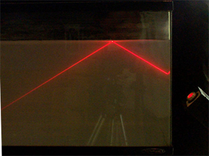
This simulation is in fact quite basic but contains all the most fundamental bricks used in more realistic photon transport simulation programs. A few things we are missing: when the photons hit the surface, some of them are actually reflected right away due to specular reflection (if there is a mismatched boundary at the slab surface). Equations for the specular reflectance are quite easy to implement. Another important thing. When photons hit the internal surface of the slab, rather than leaving the surface, they may be trapped in the slab due to internal reflectance (check the accompanying image showing a laser beam reflected at the surface of the medium). This happens when the angle of incidence is lower than the critical angle (we talked about the concept of critical angle in the lesson Interaction Light-Matter in the chapter on reflection and refraction). Internal reflectance is calculated by Fresnel's formulas (you can find them explained in the lesson on BRDF). Finally, you may want to simulate photon transport in multi-layered tissue. Check the reference section to find more details on these features.
What Have We Learned?
We have introduced a lot of new ideas and concepts in this chapter. First and foremost, this chapter was about showing an example of an unbiased Monte Carlo simulation, by simulating the transport of light/photons in tissue (the same method could be used for neutrons). To randomly sample the distance between two scattering events, we used the inverse transform sampling method which we learned about in the lesson Mathematical Foundations of Monte Carlo Methods. We showed how this works for instance with the PDF that defines the probability of a photon to either be absorbed or scattered with distance as well as with the H-G scattering phase function. We have also done some geometry to compute a new direction for the photon (and used Rodrigue's rotation formula). We introduced the concept of Russian roulette, which we will talk about in more detail in the lesson on Light Transport. Finally, we also introduced the concept of progressive rendering.
One important note to make about this Monte Carlo simulation: because the photons are independent of each other (the path that each photon follows is unique and doesn't depend on the path the other photons take), the code is highly parallelizable (so perfect for the GPU). An example of this can be done, we will be given in a future revision of this lesson.
References
Monte Carlo Modeling of Light Transport in Multi-layered Tissues in Standard C, 1992, Lihong Wang, Ph. D. Steven L. Jacques, Ph. D.
An Assessment of Laser Range Measurement on Marble Surface, 2001, G. Godin, M. Rioux, J-A Beraldin, M. Levoy, L. Cournoyer, F. Blais.
Exercises
Visualize the diffuse reflectance or the absorption (as a function of depth).
Adapt the code to the GPU. Parallelize it.
Adapt the code to work with colors. Hint: you will need to declare the absorption and the scattering coefficient as an array of three floats (one for each of the three channels R, G, and B).
Visualize in 3D the path of a few photons.