Variance Reduction Methods: a Quick Introduction to Importance Sampling
Reading time: 21 mins.The Art of Variance Reduction: Better for Less
Both variance reduction techniques and Quasi-Monte Calo methods (which we will talk about in the next chapter) are complex topics. Why should you learn about them now? People have written entire books on these topics alone. Why are they are so important? Monte Carlo as you may have realized is quite a simple method. Its main problem though is variance (in rendering, this turns into noise). To get rid of it, all we can do is increase the number of samples N, and to make things worse, each time you want to reduce this noise by two, you need not two but four times as many samples (for the error to decrease linearly, the number of samples needs to increase exponentially). Thus a great deal of research was invested into finding whether this noise could be reduced by any other means than just the brute force approach (increasing N). And it happens that mathematics again can help answer this question. This led to an entire branch in Monte Carlo research focused on what's known as variance reduction methods. How can we reduce variance by any other means than just increasing N? It happens that importance sampling and quasi-Monte Carlo are two such solutions. Of course, you can imagine why people are so excited about it. It is the Saint Graal of Monte Carlo rendering: the promise of better for less. Importance sampling and quasi-Monte Carlo deserve a lesson of their own (which you will find later in this section). Teaching these techniques will also become easier once the topic of light transport and BRDFs have been reviewed (the next three lessons). But let's briefly talk about them now, just to give you a feel of what they are how and why they work (if you are not interested in the mathematical details and just want to have an intuitive understanding of what these methods are, this introduction is probably what you are looking for and good enough).
A Quick Introduction to Importance Sampling
In the lesson Introduction to Shading, we already explained that to shade a point P, we need to gather light arriving at P. In 3D, light can come from all directions in the hemisphere oriented about the normal at P which mathematically, we can define as an integral over the hemisphere (the hemisphere is the domain of integration):
$$L = \int_\Omega L(\omega)\:d\omega.$$The symbol \(\Omega\) is usually used in the literature to denote the hemisphere of direction (and \(d\omega\) is a differential solid angle, \(\omega\) a direction) and \(L(\omega)\) a function of direction (it returns the amount of light coming from \(\omega\)). Technically, we should add a \(\cos(\theta)\) in this expression but it is not important for this demonstration. What is important, is to realize that finding how much light arrives at P requires an integral over the entire hemisphere of directions above P. Unfortunately, there is no closed form to this integral for arbitrary geometry. However, we can approximate the result of this integral with Monte Carlo integration. The idea is to "sample" the hemisphere or to create a set of N random directions over the hemisphere about P. The approximation of the integral is just an average of the amount of light coming from these N randomly chosen directions:
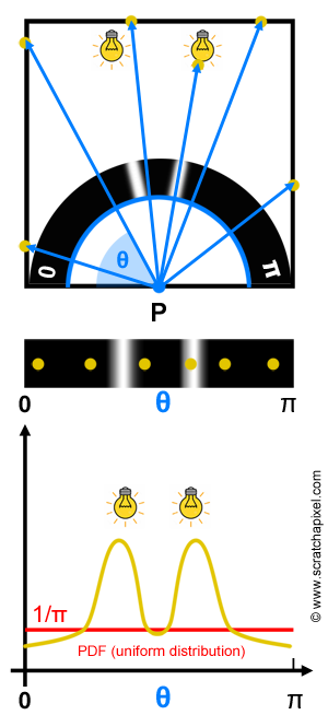
$$L \approx { 2 \pi \over N } \sum_{i=0}^{N-1} L_i(\omega_i),$$where \(\omega_i\) is a random direction contained in the hemisphere above P (in the lesson Sampling from the advanced section, you can learn how to create samples over the hemisphere). An illustration of this technique can be seen in figure 1 (top). In two dimensions though, the hemisphere becomes a half disk. Now, as with most of the Monte Carlo integration cases, we have been studying so far, the samples are uniformly distributed. In other words, each direction in the hemisphere has an equal probability to be chosen. If we consider the 2D case, the direction is reduced to an angle (\(\theta\)) going from 0 to \(\pi\). The domain of integration being defined by the interval [0,\(\pi\)], the PDF (which we know is 1/(b-a)) is therefore 1/\(\pi\) and is uniform all across i.e. the distribution function is constant (figure 1, bottom, the red line represents this PDF).
Let's now look into what the problem is. As you can see at the top of figure 1, we are trying to find out how much light arrives at P, a point located on the floor of a box. To make the demonstration easier, we will imagine that the walls of this box are very dark, therefore they will contribute very little to the illumination of P. However, we have two lights on the ceiling of this room. Naturally, most of the light illuminating the floor will come from these two light sources. But, as you can see in the figure, on the six samples used in our Monte Carlo integration to approximate light arriving at P, all samples are missing these lights but one. Since the contribution of one of the lights is missing, we can assume that the approximation of the amount of light arriving at P using this set of samples, will be underestimated. In other words, we can expect the difference between the approximation (the Monte Carlo integration) and the expected value of f(x) to be quite high (variance will be high).
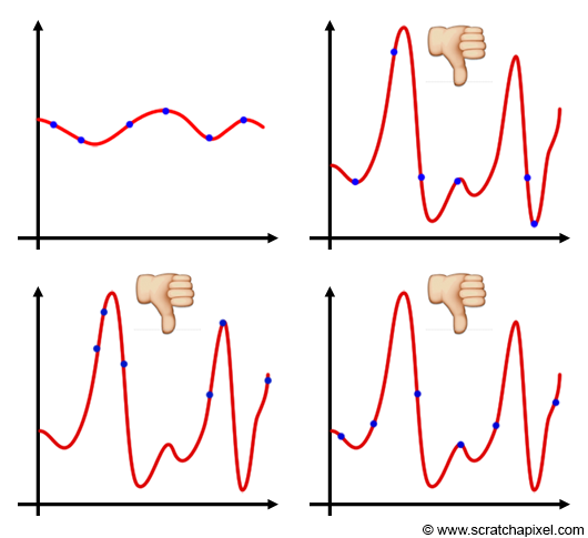
When the function is pretty regular, the position of the samples has little impact on the result. When the function is very irregular, a small change in the sample position may cause a large-scale change in the result of the Monte Carlo integration. In general, irregular functions are difficult to sample and cause a high variance in the estimator (figure 2).
Technically you can see the amount of light arriving at P as a function defined over the interval [0,\(\pi\)]. This is like rotating the hand of a watch from one side of the disk to the other, and measuring how much light strikes P from the direction pointed out by the hand. At the bottom of figure 1, you can see what this function looks like (the yellow curve). It's a nice, continuous smooth curve, with two distinct peaks one for each of the two light sources. If we were to integrate this function, in the entire domain over which this function is valid, it is pretty clear that these two peaks would have a more important contribution to the result of the integral than any other part of the curve. We can say that these peaks are where the function is the most important. As we said, it would make sense to create samples where the function is important but as we have just explained, there is no guarantee that it will be the case particularly when the sample is uniformly distributed.

Now you may think that this is not a problem. Why not just create samples where the function is important (figure 3)? There are at least two problems with this approach. First, keep in mind that Monte Carlo integration is a stochastic process. In other words, it only works because samples are chosen randomly. If you start deciding where you put the samples (rather than randomly distributing them), the theory of monte Carlo integration will fall apart (the result of your sudo Monte Carlo integration will have no mathematical meaning). Concentrating samples where the function is important while ignoring the over parts of the curve will probably overestimate the result anyway, which is not good either. But the second problem is even more critical: knowing where the function is important, suggests that we know what that function is in the first place, which obviously in most situations, is the information we don't have. For example in the example of finding how many light strikes P, we just don't know anything about where is the light coming from and in which amount. If we had this information, we would probably not use monte carlo integration in the first place anyway. We only use this method, because precisely, we don't know beforehand what that function is, so we just sample it, randomly, hoping that the average of these samples will give us a valid approximation to the integral.
This is a very important point in Monte Carlo integration. In most situations, we have no prior knowledge of the function (the integrand) being integrated, and this is often particularly true in rendering.
Another example: In the last chapter of the lesson Introduction to Shading and Radiometry, we explained that the intensity of a pixel is the result of integrating the incoming radiance over the area of this pixel. We also explained how Monte Carlo integration could be used to approximate the result of this integral. In this particular case, surfaces making up the scene and reflecting light towards the pixel, are making up the function being integrated. In this example as well, we don't know what that function is, which is obviously why we use ray tracing in the first place. We cast rays randomly distributed over the area of the pixel to sample that function, and then average the result of these rays to get an approximation to the integral.
Unfortunately, variance reduction techniques require some previous knowledge of the function being integrated. In some important cases (such as the two we described in this chapter, integrating the incoming radiance over the pixel area and the incoming light at P) we don't know what that function is. So what's the deal? Helas, there's no magical solution to this problem. If you don't have any prior knowledge of the function being integrated, just forget about variance reduction. But let's see what we can do when we know about f(x) before the integration (we will show an example related to rendering later in this chapter).
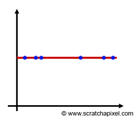
Let's imagine that the integrand is a constant function (figure 4). So you go with a uniform distribution, you sample your constant function, get a result, and everything is great. Since the function is constant, every time you run this approximation you get the same result. In other words, variance is simply zero. The ultimate goal of Monte Carlo integration is to have the smallest possible variance, with the smallest number of samples. So obviously when the variance is 0, you can't get anything better than that. Then you might think "wouldn't it be great if all functions that needed integration, were constant". Though, in reality, we know that this is never the case: functions that need integration are never constant (it would be too easy). Some of them can even have very high narrow peaks. But can we turn a nonconstant function into a constant function?
While being a rather strange thought, the answer to this question is obviously yes. You just need to divide the function by itself. If the function f(x) equals 2 when x=0, then f(0)/2 = 1. If the function f(x) = 0.5 when x = 2 then f(2)/0.5 = 1. If you do this for every value of x, then you end up with a constant function f(x)/f(x) = 1.

As we showed in figure 5 (right), dividing f(x) by another other function exactly proportional to f(x) gives a constant function as well. If \(f'(x)\) is a copy of \(f(x)\) but either scaled up or down by a constant factor \(c\), we have:
$$f(x) = c f'(x),$$and thus:
$$\dfrac{f(x)}{f'(x) } = \dfrac{1}{c}.$$Now you will think, that's great and simple but what's the point, since the function we are interested in is f(x) and not a constant function? That's true, but have another look at the formula for the general Monte Carlo estimator again:
$$\langle F^N \rangle = \dfrac{1}{N} \sum_{i=0}^{N-1} {\dfrac{\color{orange}{f(x)}}{\color{red}{pdf(x)}}}.$$We kept the same color code (red for f(x) and yellow for f'(x)) so that you can more easily see where we are heading at. In the Monte Carlo estimator, the integrand f(x) is divided by another function, pdf(x). Taking advantage of what we just learned, if pdf(x) is a function exactly proportional to f(x), then the variance of the Monte Carlo integral will also exactly be 0!
Since Monte Carlo integration applied to a constant function has no variance (regardless of the way samples are distributed), we can take advantage of the general Monte Carlo estimator (in which the integrand f(x) is divided by pdf(x)) to create the same effect. Indeed, if the pdf(x) (in the numerator) is a function whose shape is exactly proportional (the ideal case) or as similar as possible to the integrand, then variance will either be 0 (the ideal case) or potentially greatly reduced:
$${\dfrac{\color{black}{f(x) }}{\color{red}{pdf(x)}}} = {\dfrac{\color{black}{ f(x) }}{\color{red}{c \:f(x)}}} = \dfrac{1}{c}.$$What it means in practice, is that to reduce variance, our task is to find a pdf that is matching as closely as possible the shape of the integrand. When the PDF matches the shape of the function exactly, you can be a perfect estimator.

This is not always possible, because as we said before, we don't always know what f(x) looks like. However, when we do, variance reduction can be achieved, by selecting a pdf whose shape is similar to the shape of f(x) (this is often possible in shading). This idea is illustrated in Figure 6 in which the integrand function is plotted in blue and the pdf in red. If we don't know anything about the function's shape, our best choice is probably to stick with a uniform distribution. Of course, it won't be as good as if the pdf and the integrand had a similar shape (Figure 6, middle) but certainly still better than if we choose a pdf whose shape is different than the function (as shown in the bottom of Figure 6). In summary, if you don't know what f(x) looks like or if you don't know how to build a pdf to match the shape of f(x), just stick to a uniform distribution. But at all costs, avoid using a pdf which is very different than f(x), because instead of reducing variance, you will do the exact opposite, which is to likely increase it a great deal. And remember, noise is what we try to get rid of so let's not add any more of it!
How do we choose the pdf? This part will be detailed in the lesson Importance Sampling.
Before we look at a simple example (practical examples applied to rendering will be given in the lesson on importance sampling), let's explain where the term importance sampling comes from. In the chapter on Monte Carlo simulation, we introduced the general formula of the Monte Carlo estimator, in which the integrand is divided by the pdf. If the PDF is nonuniform, the density of samples may vary across the domain of integration (creating more samples in areas where the PDF is high, and less where it is low). One important observation is that, if the PDF has more or less the same shape as the integrand f(x), then using this PDF will generate more samples in areas where the function is also important.
By choosing a PDF whose shape is similar to that of the integrand f(x), we generate more samples where the function is also likely to be important. Whenever we will have prior knowledge of f(x) we will attempt to choose a pdf(x) with exactly or approximately the same shape as the integrand. Using this PDF to generate our samples (sampling the random variable X from this pdf) will generate more samples where f(x) is important, thus reducing the risk of missing the important features of the function, and consequently reducing variance. Hence the term importance sampling. We distribute more samples wherever the function f(x) is important, while still eventually distributing samples (only less) wherever the function is less important
So in essence it's like combining the best of two worlds: we still have a stochastic process in which samples are chosen randomly, only they are distributed from a given PDF, so more samples might be generated where the pdf is high, etc. But, while choosing this PDF wisely, we can reduce variance, by reducing the "chance" of missing the important features of the function (and these features are important because they contribute the most to the result of the integral).
Remember from our initial example, that our problem was that on 6 samples, only 1 was sampling one of the two peaks. Because the contribution of one of the peaks is ignored, the error is high. However, with importance sampling, assuming we can create a PDF that has a similar shape to our yellow curve, then we increase our chances to see more samples around these two peaks, thus potentially reducing variance (the error between the approximation and the expected value of f(x)).
In the chapter on Monte Carlo integration, we proved that the expected value of the MC general estimator formula is indeed equal to the expected value of f(x). However, remember that we also gave an intuitive explanation of the process. Because sampling the random variables from an arbitrary PDF, generates more samples in some areas and fewer in others, dividing f(x) by the pdf, reduces the contribution or weight of samples generated in areas of higher density and increases the contribution of those generated in areas of lesser density.
So again, by generating samples where the function is important, we reduce the variance, however, we have also proven that the formula is mathematically valid and leads to the correct solution (which is that as the number of samples increases, the Monte Carlo integration will eventually converge to the expected value of f(x)).
Also an important note. Notice that even though more samples are generated in regions where the function is important, the process stays stochastic. Not only where the samples will be generated can't be determined ahead, but it's not because we can expect more samples to be generated where the PDF is high (we can't know for sure, since the samples are drawn randomly, but statistically we have more chances to see them generated in these regions), that no samples will be generated at all where the PDF is low.
Again, it's about the art of distributing our credit of samples in the most efficient way, devoting a good chunk of them into sampling the function where it is high or important (it contributes the most to the integral) while keeping a few to sample the function everywhere else. The art of Monte Carlo integration is to find the optimal solution to this problem. Where should I invest my samples in, to get the smallest possible error for a fixed number of samples N?
Our goal is to compute an approximation of the integral: \(I = \int_a^b f(x) \; dx\). The function \(p(x)\) is a probability distribution function defined over the interval [a,b], and \(\xi\) is a random variable defined over the interval [a,b] with density \(p(x)\).
Let's write: \(\eta = \dfrac{f(\xi)}{p(\xi)}\),
where \(\eta\) is also a random variable. Since we know that the expected value of a function of a random variable is \(E[f(x)] = \int_a^b f(x) p(x)\;dx\), we can write:
$$E[\eta] = E\left[\dfrac{f(\xi)}{p(\xi)}\right] = \int_a^b \dfrac{f(x)}{p(x)} p(x) \;dx = \int_a^b f(x) \; dx = I.$$Example

Finally, let's look at a simple example. We use Monte Carlo integration to approximate the following integral:
$$F = \int_0^{\pi \over 2} \sin(x) \; dx.$$The great thing about this function is that we can compute the result of the integral analytically using the second fundamental theorem of calculus (see the chapter Mathemmatics of Shading in the lesson Introduction to Shading & Radiometry). The antiderivative of \(\sin(x)\) is \(-\cos(x)\). Thus we can write:
$$F = \left[ -\cos(x) \right]_0^{\pi \over 2} = -\cos(\dfrac{\pi}{2}) - - \cos(0) = 1.$$The result of this integral is 1\. Now we will try to approximate this integral using Monte Carlo integration. We will be using two different pdfs a uniform probability distribution (\(p(x) = 2 / \pi x\)) and a pdf (\(p'(x) = 8x/\pi^2\)) which as you can see in figure 7, has a shape that matches the shape of the integrand better than the uniform PDF. The theory tells us that drawing samples from this PDF should reduce the variance compared to drawing samples from the uniform PDF. Let's check it then! For the uniform distribution, we will be using the following estimator:
$$\langle F^N \rangle = \dfrac{(\pi / 2)}{N} \sum_{i=0}^{N-1} sin(X_i),$$where the \(X_i\)s are drawn from a PDF with uniform distribution. As for the second PDF, let's use the inverse sampling method to find the formula we will be using to draw samples. Recall that we first need to compute and then invert the CDF.
$$CDF(x < \mu) = \int_0^\mu {\dfrac{8x} {\pi^2}} = \left[ {\dfrac{4x^2}{\pi^2}} \right]_0^\mu = {\dfrac{4\mu^2}{\pi^2}} - 0.$$Now, let's invert the function:
$$ \begin{array}{l} \xi &=& \dfrac{4x^2}{\pi^2},\\ x^2 & = &\dfrac{\pi^2}{4} \xi,\\ x &=& \dfrac{\pi}{2}\sqrt{\xi}. \end{array} $$Let's now implement these formulas in a program and compare the results:
#include <cstdio>
#include <cstdlib>
#include <cmath>
int main(int argc, char **argv)
{
    srand48(13);
    int N = 16;
    for (int n = 0; n < 10; ++n) {
        float sumUniform = 0, sumImportance = 0;
        for (int i = 0; i < N; ++i) {
            float r = drand48();
            sumUniform += sin(r * M_PI * 0.5);
            float xi = sqrtf(r) * M_PI * 0.5;  //this is our X_i
            sumImportance += sin(xi) / ((8 * xi) / (M_PI * M_PI));
        }
        sumUniform *= (M_PI * 0.5) / N;
        sumImportance *= 1.f / N;
        printf("%f %f\n", sumUniform, sumImportance);
    }
    return 0;
}
If you run the program you should get the following results (with N = 16):
# |
Uniform |
Importance |
Err. Uniform % |
Err. Importance % |
|---|---|---|---|---|
0 |
1.125890 |
0.969068 |
12% |
-3% |
1 |
1.277833 |
0.925675 |
27% |
-7% |
2 |
1.054394 |
0.980940 |
5% |
-1% |
3 |
1.022417 |
0.989288 |
2% |
-1% |
4 |
1.231261 |
0.936890 |
23% |
-6% |
5 |
0.830151 |
1.041751 |
-16% |
4% |
6 |
1.062268 |
0.989363 |
6% |
-1% |
7 |
0.849265 |
1.043809 |
-15% |
4% |
8 |
0.921527 |
1.020279 |
-7% |
2% |
9 |
1.002310 |
0.994284 |
0% |
0% |

You can see in the last two columns, where variance is expressed as a percentage (of the difference between the result of the Monte Carlo integration and the actual expected value of f(x) which we know is 1), that the error is greater on average with uniform sampling than it is with importance sampling (rightmost column). As a side note, note how the last run (last row) gives a result very close to the correct solution (for both methods). This is a good example of what we explained in the first chapter of this lesson: because we use random samples, an MC method can as well "just" randomly falls on the exact value by pure chance (on some occasions).
This concludes our "short" introduction to importance sampling. This example is very simple; its aim is just to show that it works. In the lesson Importance Sampling, you will find more complex examples which also apply more directly to rendering.