3D Viewing: the Pinhole Camera Model

Implementing a Virtual Pinhole Camera

Implementing a Virtual Pinhole Camera Model

In the last three chapters, we have learned everything there is to know about the pinhole camera model. This type of camera is the simplest to simulate in CG and is the model most commonly used by video games and 3D applications. As briefly mentioned in the first chapter, pinhole cameras, by their design, can only produce sharp images (without any depth of field). While simple and easy to implement, the model is also often criticized for not being able to simulate visual effects such as depth of field or lens flare. While some perceive these effects as visual artifacts, they play an important role in the aesthetic experiences of photographs and films. Simulating these effects is relatively easy (because it essentially relies on well-known and basic optical rules) but very costly, especially compared to the time it takes to render an image with a basic pinhole camera model. We will present a method for simulating depth of field in another lesson (which is still costly but less costly than if we had to simulate depth of field by following the path of light rays through the various optics of a camera lens).

In this chapter, we will use everything we have learned in the previous chapters about the pinhole camera model and write a program to implement this model. To convince you that this model works and that there is nothing mysterious or magical about how images are produced in software such as Maya. We will produce a series of images by changing different camera parameters in Maya and our program and compare the results. If all goes well, when the camera settings match, the two applications' images should also match. Let's get started.

Implementing an Ideal Pinhole Camera Model

When we refer to the pinhole camera in the rest of this chapter, we will use the terms focal length and film size. Please distinguish them from the near-clipping plane and the canvas size terms. The former applies to the pinhole camera, and the latter applies to the virtual camera model only. However, they do relate to each other. Let's quickly explain again how.

The pinhole and virtual cameras must have the same viewing frustum to deliver the same image. The viewing frustum itself is defined by two and only two parameters: the point of convergence, the camera or eye origin (all these terms designate the same point), and the angle of view. We also learned in the previous chapters that the angle of view was defined by the film size and the focal length, two parameters of the pinhole camera.

Where Shall the Canvas/Screen Be?

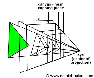
In CG, once the viewing frustum is defined, we then need to define where is the virtual image plane going to be. Mathematically though, the canvas can be anywhere we want along the line of sight, as long as the surface on which we project the image is contained within the viewing frustum, as shown in Figure 1; it can be anywhere between the apex of the pyramid (obviously not the apex itself) and its base (which is defined by the far clipping plane) or even further if we wanted to.

When the distance between the eye and the image plane is equal to 1, it is convenient because it simplifies the equations to compute the coordinates of a point projected on the canvas. However, if we were making that choice, we wouldn't have the opportunity to study the generic (and slightly more complex) case in which the distance to the canvas is arbitrary. And since our goal on Scratchapixel is to learn how things work rather than make our life easier, let's skip this option and choose the generic case instead. For now, we decided to position the canvas at the near-clipping plane. Refrain from trying to make any sense as to why we decide to do so. It is only motivated by pedagogical reasons. The near-clipping plane is a parameter that the user can change by setting the image plane at the near-clipping plane; this forces us to study the equations for projecting points on a canvas located at an arbitrary distance from the eye. We are also cheating slightly because the way the perspective projection matrix works is based on implicitly setting up the image plane at the near-clipping plane. Thus by making this choice, we also anticipate what we will study in the next lesson. However, remember that where the canvas is positioned does not affect the output image (the image plane can be located between the eye and the near-clipping plane. Objects between the eye and the near clipping plane could still be projected on the image plane; equations for the perspective matrix would still work).

What Will our Program Do

In this lesson, we will create a program to generate a wireframe image of a 3D object by projecting the object's vertices onto the image plane. The program will be very similar to the one we wrote in the previous lesson; we will now extend the code to integrate the concept of focal length and film size. Film formats are generally rectangular, not square. Thus, our program will also output images with a rectangular shape. Remember that in chapter 2, we mentioned that the resolution gate aspect ratio, also called the device aspect ratio (the image width over its height), was not necessarily the same as the film gate aspect ratio (the film width over its height). In the last part of this chapter, we will also write some code to handle this case.

Here is a list of the parameters our pinhole camera model will require:

Intrinsic Parameters

Extrinsic Parameters

We will also need the following parameters, which we can compute from the parameters listed above:

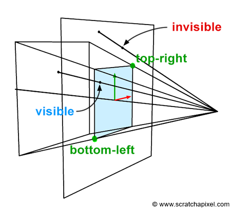
Remember that when a 3D point is projected onto the image plane, we need to test the projected point x- and y-coordinates against the canvas coordinates to find out if the point is visible in the camera's view or not. Of course, the point can only be visible if it lies within the canvas limits. We already know how to compute the projected point coordinates using perspective divide. But we still need to know the canvas's bottom-left and top-right coordinates (Figure 2). How do we find these coordinates, then?

In almost every case, we want the canvas to be centered around the canvas coordinate system origin (Figures 2, 3, and 4). However, this is only sometimes or doesn't have to be the case. A stereo camera setup, for example, requires the canvas to be slightly shifted to the left or the right of the coordinate system origin. Therefore, this lesson will always assume that the canvas is centered on the image plane coordinate system origin.

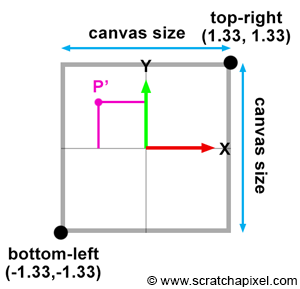
Computing the canvas or screen window coordinates is simple. Since the canvas is centered about the screen coordinate system origin, they are equal to half the canvas size. They are negative if they are either below or to the left of the y-axis and x-axis of the screen coordinate system, respectively (Figure 4). The canvas size depends on the angle of view and the near-clipping plane (since we decided to position the image plane at the near-clipping plane). The angle of view depends on the film size and the focal length. Let's compute each one of these variables.

Note, though, that the film format is more often rectangular than square, as mentioned several times. Thus the angular horizontal and vertical extent of the viewing frustum is different. So we will need the horizontal angle of view to compute the left and right coordinates and the vertical angle of view to compute the bottom and top coordinates.

Computing the Canvas Coordinates: The Long Way

Let's start with the horizontal angle of view. In the previous chapters, we introduced the equation to compute the angle of view. It can easily be done using trigonometric identities. If you look at the camera setup from the top, you can see that we can trace a right triangle (Figure 6). The adjacent and opposite sides of the triangles are known: they correspond to the focal length and half of the film's horizontal aperture. However, they must be defined in the same unit to be used in a trigonometric identity. Typically, film gate dimensions are defined in inches, and focal length is defined in millimeters. Generally, inches are converted into millimeters, but you can convert millimeters to inches if you prefer; the result will be the same. One inch corresponds to 25.4 millimeters. To find the horizontal angle of view, we will use a trigonometric identity that says that the tangent of an angle is the ratio of the length of the opposite side to the length of the adjacent side (equation 1):

Where \(\theta_H\) is the horizontal angle of view, we can compute the canvas size now that we have theta. We know it depends on the angle of view and the near-clipping plane (because the canvas is positioned at the near-clipping plane). We will use the same trigonometric identity (Figure 6) to compute the canvas size (equation 2):

If we want to avoid computing the trigonometric function tan(), we can substitute the function on the right-hand side of equation 1:

To compute the right coordinate, we need to divide the whole equation by 2. We get:

Computing the left is trivial. For example, here is a code fragment to compute the left and right coordinates:

float focalLength = 35;
// 35mm Full Aperture
float filmApertureWidth = 0.980;
float filmApertureHeight = 0.735;
static const float inchToMm = 25.4;
float nearClippingPlane = 0.1;
float farClipingPlane = 1000;

int main(int argc, char **argv)
{
#if 0
    // First method. Compute the horizontal angle of view first
    float angleOfViewHorizontal = 2 * atan((filmApertureWidth * inchToMm / 2) / focalLength);
    float right = tan(angleOfViewHorizontal / 2) * nearClippingPlane;
#else
    // Second method. Compute the right coordinate directly
    float right = ((filmApertureWidth * inchToMm / 2) / focalLength) * nearClippingPlane;
#endif

    float left = -right;

    printf("Screen window left/right coordinates %f %f\n", left, right);

    ...
}

We can use the same technique to compute the top and bottom coordinates, only this time; we need to compute the vertical angle of view (\(\theta_V\)):

We can then find the equation for the top coordinate:

Here is the code to compute all four coordinates:

int main(int argc, char **argv)
{
#if 0
    // First method. Compute the horizontal and vertical angle of view first
    float angleOfViewHorizontal = 2 * atan((filmApertureWidth * inchToMm / 2) / focalLength);
    float right = tan(angleOfViewHorizontal / 2) * nearClippingPlane;
    float angleOfViewVertical = 2 * atan((filmApertureHeight * inchToMm / 2) / focalLength);
    float top = tan(angleOfViewVertical / 2) * nearClippingPlane;
#else
    // Second method. Compute the right and top coordinates directly
    float right = ((filmApertureWidth * inchToMm / 2) / focalLength) * nearClippingPlane;
    float top = ((filmApertureHeight * inchToMm / 2) / focalLength) * nearClippingPlane;
#endif

    float left = -right;
    float bottom = -top;

    printf("Screen window bottom-left, top-right coordinates %f %f %f %f\n", bottom, left, top, right);
    ...
}

Computing the Canvas Coordinates: The Quick Way

The code we wrote is working just fine. However, there is a slightly faster way of computing the canvas coordinates (which you will likely see being used in production code). The method consists of computing the vertical angle of view to get the bottom-top coordinates, and they multiply these coordinates by the film aspect ratio. Mathematically this is working because this comes back to writing:

The following code shows how to implement this solution:

int main(int argc, char **argv)
{
    float top = ((filmApertureHeight * inchToMm / 2) / focalLength) * nearClippingPlane;
    float bottom = -top;
    float filmAspectRatio = filmApertureWidth / filmApertureHeight;
    float left = bottom * filmAspectRatio;
    float left = -right;

    printf("Screen window bottom-left, top-right coordinates %f %f %f %f\n", bottom, left, top, right);
    ...
}

Does it Work? Checking the Code

Before we test the code, we need to make a slight change to the function that projects points onto the image plane. Remember that to compute the projected point coordinates; we use a property of similar triangles. For example, if A, B, A' and B' are the opposite and adjacent sides of two similar triangles, then we can write:

In the previous lesson, we positioned the canvas 1 unit away from the eye. Thus the near clipping plane was equal to 1, and it reduced the equation to a simple division of the point x- and y-coordinates by the point z-coordinate (in other words, we ignored \\(Z\_{near}\\)). We will also test whether the point is visible in the function to compute the projected point coordinates. We will compare the Finally, projected point coordinates with the canvas coordinates. In the program, if any of the triangle's vertices are outside the canvas boundaries, we will draw the triangle in red (if you see a red triangle in the image, then at least one of its vertices lies outside the canvas). Here is an updated version of the function projecting points onto the canvas and computing the raster coordinates of a 3D point:

bool computePixelCoordinates(
    const Vec3f &pWorld,
    const Matrix44f &worldToCamera,
    const float &b,
    const float &l,
    const float &t,
    const float &r,
    const float &near,
    const uint32_t &imageWidth,
    const uint32_t &imageHeight,
    Vec2i &pRaster)
{
    Vec3f pCamera;
    worldToCamera.multVecMatrix(pWorld, pCamera);
    Vec2f pScreen;
    pScreen.x = pCamera.x / -pCamera.z * near;
    pScreen.y = pCamera.y / -pCamera.z * near;

    Vec2f pNDC;
    pNDC.x = (pScreen.x + r) / (2 * r);
    pNDC.y = (pScreen.y + t) / (2 * t);
    pRaster.x = (int)(pNDC.x * imageWidth);
    pRaster.y = (int)((1 - pNDC.y) * imageHeight);

    bool visible = true;
    if (pScreen.x < l || pScreen.x > r || pScreen.y < b || pScreen.y > t)
        visible = false;

    return visible;
}

Here is a summary of the changes we made to the function:

• Lines 16 and 17: the result of the perspective divide is multiplied by the near-clipping plane.

• Lines 20 and 21: to remap the point from screen space to NDC space, we divide the point x and y-coordinates in screen space by the canvas width and height, respectively.

• Lines 26 and 27: the point coordinates in screen space are compared with the bottom-left, top-right canvas coordinates. If the point lies outside, we set the visible variable to false.

The rest of the program (which you can find in the source code section) is similar to the previous program. We loop over all the triangles of the 3D model, convert the triangle's vertices coordinates to raster coordinates and store the result in an SVG file. Let's render a few images in Maya and with our program and check the results.

As you can see, the results match. Maya and our program produce the same results (the size and position of the model in the images are consistent between applications). When the triangles overlap the canvas boundaries, they are red, as expected.

When the Resolution Gate and Film Gate Ratio Don't Match

When the film gate aspect ratio and the resolution gate aspect ratio (also called device aspect ratio) are different, we need to decide whether we fit the resolution gate within the film gate or the other way around (the film gate is fit to match the resolution gate). Let's check what the different options are:

• Fill Mode: we fit the resolution gate within the film gate (the blue box is contained within the red box). We have to handle two cases:

  • Figure 8a: when the film aspect ratio is greater than the device aspect ratio, the canvas left, and right coordinates need to be scaled down to match the left and right coordinates of the resolution gate. This can be done by multiplying the left and right coordinates by the resolution aspect ratio over the film aspect ratio.

  • Figure 8c: when the film aspect ratio is lower than the device aspect ratio, the canvas top and bottom coordinates need to be scaled down to match the top and bottom coordinates of the resolution gate. This can be done by multiplying the top and bottom coordinates by the film aspect ratio over the resolution aspect ratio.

• Overscan Mode: we fit the film gate within the resolution gate (the red box is contained within the blue box). We have to handle two cases:

  • Figure 8b: when the film aspect ratio is greater than the device aspect ratio, the canvas top and bottom coordinates need to be scaled up to match the resolution gate top and bottom coordinates. To do so, we multiply the canvas top and bottom coordinates by the film aspect ratio over the resolution aspect ratio.

  • Figure 8d: when the film aspect ratio is lower than the device aspect ratio, the canvas left, and right coordinates need to be scaled up to match the resolution gate top and bottom coordinates. To do so, we multiply the canvas top and bottom coordinates by the resolution aspect ratio over the film aspect ratio.

The following code fragment demonstrates how you can implement these four cases:

float xscale = 1;
float yscale = 1;

switch (fitFilm) {
    default:
    case kFill:
        if (filmAspectRatio > deviceAspectRatio) {
            // 8a
            xscale = deviceAspectRatio / filmAspectRatio;
        }
        else {
            // 8c
            yscale = filmAspectRatio / deviceAspectRatio;
        }
        break;
    case kOverscan:
        if (filmAspectRatio > deviceAspectRatio) {
            // 8b
            yscale = filmAspectRatio / deviceAspectRatio;
        }
        else {
            // 8d
            xscale = deviceAspectRatio / filmAspectRatio;
        }
        break;
}

right *= xscale;
top *= yscale;
left = -right;
bottom = -top;

Check the next chapter to get the source code of the complete program.

Conclusion

In this lesson, you have learned everything there is to know about simulating a pinhole camera in CG. In the process, we also learned how to project points onto the image plane and find if they are visible to the camera by comparing their coordinates to the canvas coordinates. The concepts learned in this lesson will be useful for studying the perspective projection matrix (the next lesson's topic), the REYES algorithm, a popular rasterization algorithm, and how images are formed in ray tracing.