The Pinhole Camera Model

A Virtual Pinhole Camera Model

Our next step is to develop a virtual camera based on the same principles as a pinhole camera. More precisely, our goal is to create a camera model that delivers images similar to those produced by a real pinhole camera. For example, if we take a picture of a given object with a pinhole camera, then when a 3D replica of that object is rendered with our virtual camera, the size and shape of the object in the computer-generated (CG) render must exactly match the size and shape of the real object in the photograph. However, before delving into the model itself, it is important to learn more about computer graphics camera models.

First, the details:

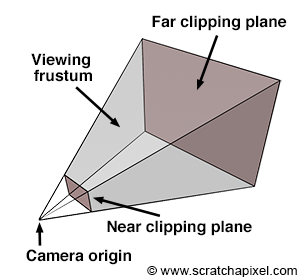
• CG cameras have near and far clipping planes. Objects closer than the near clipping plane or farther than the far clipping plane are invisible to the camera. This feature allows us to exclude some scene geometry and render only specific portions of the scene, which is essential for rasterization to work.

• In this chapter, we will also explore why, in CG, the image plane is positioned in front of the camera's aperture rather than behind it, as with real pinhole cameras. This positioning plays a crucial role in how cameras are conventionally defined in CG.

• Finally, we must examine how to render a scene from any given viewpoint. Although this topic was discussed in the previous lesson, this chapter will briefly revisit it.

The important question we haven't yet addressed is, "Studying real cameras to understand how they work is great, but how is the camera model used to produce images?" In this chapter, we will demonstrate that the answer to this question depends on whether we use rasterization or ray-tracing as the rendering technique.

In this chapter, we will first review the points listed above one by one to provide a complete "picture" of how cameras work in CG. Then, the virtual camera model will be introduced and implemented in a program in the next (and final) chapter of this lesson.

How Do We Represent Cameras in the CG World?

Photographs produced by real-world pinhole cameras are upside down. This occurs because, as explained in the first chapter, the film plane is located behind the center of projection. However, this can be avoided if the projection plane lies on the same side as the scene, as shown in Figure 1. In the real world, the image plane cannot be located in front of the aperture because it would be impossible to isolate it from unwanted light. However, in the virtual world of computers, constructing our camera in this manner is feasible. Conceptually, this construction leads to viewing the hole of the camera (which also serves as the center of projection) as the actual position of the eye, with the image plane being the image that the eye sees.

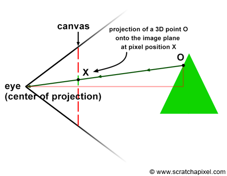
Defining our virtual camera in this way clarifies how constructing an image by following light rays from any point in the scene to the eye becomes a simple geometrical problem, known as perspective projection. Perspective projection is a method for creating an image through this apparatus, a sort of pyramid whose apex is aligned with the eye and whose base defines the surface of a canvas onto which the image of the 3D scene is "projected."

Near and Far Clipping Planes and the Viewing Frustum

The near and far clipping planes are virtual boundaries set in front of the camera, parallel to the image plane where the image is formed. These planes are positioned along the camera's line of sight, aligning with the camera's local z-axis. Unlike anything in the real world, these clipping planes play a crucial role in virtual camera models, dictating what portions of the scene are visible. Objects positioned closer than the near clipping plane or beyond the far clipping plane are rendered invisible by the camera. This concept is especially significant for scanline renderers, like OpenGL, that employ the z-buffer algorithm. These renderers use clipping planes to manage the depth value range, aiding in projecting scene points onto the image plane. Moreover, adjusting these clipping planes can alleviate precision issues, such as z-fighting, which we'll explore in the next lesson. Notably, ray tracing does not inherently require clipping planes for its operations.

The Near Clipping Plane and the Image Plane

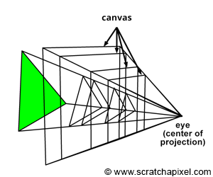
The canvas, also known as the screen in some computer graphics texts, represents the 2D surface within the image plane where the scene's image is projected. Conventionally, we might place this canvas 1 unit away from the eye, a decision simplifying the projection equations. However, as illustrated in Figure 3, the position of the canvas along the camera's local z-axis is flexible, impacting neither the image's projection nor its requirement to maintain a fixed distance from the eye. The concept of the viewing frustum, a truncated pyramid shaped by the near and far clipping planes, underscores the scene portion visible through the camera. A common approach in computer graphics involves remapping points within this frustum to a unit cube, laying the groundwork for the perspective projection matrix discussed in upcoming lessons. This technique underscores why positioning the image plane near the clipping plane is advantageous.

For the remainder of this lesson, we will assume the canvas (or screen) is located at the near-clipping plane, an arbitrary yet practical decision. This placement does not constrain the projection equations we will explore, which remain valid regardless of the canvas's specific position along the camera's z-axis, as depicted in Figure 4.

It's important to differentiate between the distance from the eye to the canvas, the near clipping plane, and the focal length. This distinction will be elaborated upon in the subsequent chapter, further clarifying the intricacies of camera modeling in computer graphics.

Computing the Canvas Size and the Canvas Coordinates

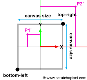
In the previous section, we emphasized the fact that the canvas's position along the camera's local z-axis affects its size. When the distance between the eye and the canvas decreases, the canvas gets smaller; conversely, when that distance increases, it gets larger. The bottom-left and top-right coordinates of the canvas are directly linked to the canvas size. Once we know the size, computing these coordinates is straightforward, considering the canvas (or screen) is centered on the origin of the image plane coordinate system. These coordinates are crucial because they allow us to easily check whether a point projected on the image plane lies within the canvas and is, therefore, visible to the camera. Figures 5, 6, and 7 project two points onto the canvas. One of them (P1') is within the canvas limits and visible to the camera, while the other (P2') is outside the boundaries and thus invisible. Knowing both the canvas coordinates and the projected coordinates makes testing the visibility of the point simple.

Let's explore how to mathematically compute these coordinates. In the second chapter of this lesson, we presented the equation to compute the canvas size (assuming the canvas is square as depicted in Figures 3, 4, and 6):

Where $\theta$ is the angle of view (hence the division by 2). Note that the vertical and horizontal angles of view are the same when the canvas is square. Since the distance from the eye to the canvas is defined as the near clipping plane, we can write:

Where $Z_{near}$ is the distance between the eye and the near-clipping plane along the camera's local z-axis, as illustrated in Figure 5. Given that the canvas is centered on the origin of the image plane coordinate system, computing the canvas's corner coordinates is straightforward. First, we divide the canvas size by 2 and set the sign of the coordinate based on the corner's position relative to the origin of the coordinate system:

Knowing the bottom-left and top-right canvas coordinates, we can compare the projected point coordinates with these values (first, we need to compute the point's coordinates on the image plane, positioned at the near clipping plane, a process we will learn in the next chapter). A point lies within the canvas boundary (and is therefore visible) if its x and y coordinates are either greater than or equal to the bottom-left and less than or equal to the top-right canvas coordinates, respectively. The following code fragment computes the canvas coordinates and tests the visibility of a point lying on the image plane against these coordinates:

// This code prioritizes clarity over optimization to enhance understanding.
// Its purpose is to elucidate rather than obscure.
float canvasSize = 2 * tan(angleOfView * 0.5) * Znear;
float top = canvasSize / 2;
float bottom = -top;
float right = canvasSize / 2;
float left = -right;
// Compute the projected point coordinates.
Vec3f Pproj = ...;
if (Pproj.x < left || Pproj.x > right || Pproj.y < bottom || Pproj.y > top) {
    // The point is outside the canvas boundaries and is not visible.
}
else {
    // The point is within the canvas boundaries and is visible.
}

Camera to World and World to Camera Matrix

Finally, we need a method to produce images of objects or scenes from any viewpoint. We discussed this topic in the previous lesson, but we will cover it briefly in this chapter. CG cameras are similar to real cameras in that respect. However, in CG, we look at the camera's view (the equivalent of a real camera viewfinder) and move around the scene or object to select a viewpoint ("viewpoint" is the camera position in relation to the subject).

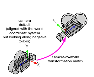
When a camera is created, by default, it is located at the origin and oriented along the negative z-axis (Figure 8). This orientation is explained in detail in the previous lesson. By doing so, the camera's local and world coordinate systems' x-axis point in the same direction. Therefore, defining the camera's transformations with a 4x4 matrix is convenient. This 4x4 matrix, which is no different from the 4x4 matrices used to transform 3D objects, is called the camera-to-world transformation matrix (because it defines the camera's transformations with respect to the world coordinate system).

The camera-to-world transformation matrix is used differently depending on whether rasterization or ray tracing is being used:

• In rasterization, the inverse of the matrix (the world-to-camera 4x4 matrix) is used to convert points defined in world space to camera space. Once in camera space, we can perform a perspective divide to compute the projected point coordinates in the image plane. An in-depth description of this process can be found in the previous lesson.

• In ray tracing, we build camera rays in the camera's default position (the rays' origin and direction) and then transform them with the camera-to-world matrix. The full process is detailed in the "Ray-Tracing: Generating Camera Rays" lesson.

Don't worry if you still don't understand how ray tracing works. We will study rasterization first and then move on to ray tracing next.

Understanding How Virtual Cameras Are Used

At this point in the lesson, we have explained almost everything there is to know about pinhole cameras and CG cameras. However, we still need to explain how images are formed with these cameras. The process depends on whether the rendering technique is rasterization or ray tracing. We are now going to consider each case individually.

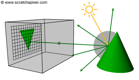
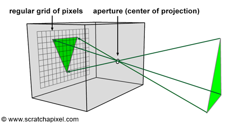
Before we do so, let's briefly recall the principle of a pinhole camera again. When light rays emitted by a light source intersect objects from the scene, they are reflected off the surface of these objects in random directions. For each point of the scene visible by the camera, only one of these reflected rays will pass through the aperture of the pinhole camera and strike the surface of the photographic paper (or film or sensor) in one unique location. If we divide the film's surface into a regular grid of pixels, what we get is a digital pinhole camera, which is essentially what we want our virtual camera to be (Figures 9 and 10).

This is how things work with a real pinhole camera. But how does it work in CG? In CG, cameras are built on the principle of a pinhole camera, but the image plane is in front of the center of projection (the aperture, which in our virtual camera model we prefer to call the eye), as shown in Figure 11. How the image is produced with this virtual pinhole camera model depends on the rendering technique. First, let's consider the two main visibility algorithms: rasterization and ray tracing.

Rasterization

In this chapter, we need to explain how the rasterization algorithm works. To gain a complete overview of the algorithm, you are encouraged to read the lesson devoted to the REYES algorithm, a widely recognized rasterization algorithm. Next, we will explore how the pinhole camera model is applied in this rendering technique. Recall that each ray passing through the aperture of a pinhole camera strikes the film's surface at a single location, which corresponds to a pixel in the context of digital images.

Consider a specific ray, R, reflected off an object's surface at point O, traveling towards the eye in direction D, passing through the camera's aperture at point A, and striking the image plane at pixel location X (Figure 12). To simulate this process, we need to compute the pixel within an image that any given light ray strikes and record the color of this light ray (the color at the point where the ray was emitted from, which essentially is the information carried by the light ray itself) at that pixel location.

This process equates to calculating the pixel coordinates X of the 3D point O using perspective projection. Perspective projection determines the position of a 3D point on the image plane by computing the intersection of a line from the point to the eye with the image plane. The method for computing this intersection point was described in detail in the previous lesson. In the next chapter, we will learn how to compute these coordinates when the canvas is positioned at an arbitrary distance from the eye (previously, the distance between the eye and the canvas was assumed to be constant at 1).

If you're still unclear about how rasterization works, don't worry too much at this point. As mentioned before, an entire lesson is devoted to this topic. The key takeaway from that lesson is the method of "projecting" 3D points onto the image plane and calculating the pixel coordinates of the projected points. This method will be our focus when working with rasterization. The projection process can be viewed as simulating how an image is formed inside a pinhole camera by "tracing" the path of light rays from their emission points in the scene to the eye and "recording" the position (in terms of pixel coordinates) where these rays intersect the image plane. This process involves transforming points from world space to camera space, performing a perspective divide to compute their coordinates in screen space, converting these coordinates to NDC space, and finally, translating these coordinates from NDC space to raster space. We applied this method in a previous lesson to produce a wireframe image of a 3D object.

for each point in the scene {
    transform a point from world space to camera space;
    perform perspective divide (x/-z, y/-z);
    if point lies within canvas boundaries {
        convert coordinates to NDC space;
        convert coordinates from NDC to raster space;
        record point in the image;
    }
}
// connect projected points to recreate the object's edges
...

In this technique, the image is formed by a collection of points (conceptually defined as the locations where light rays are reflected off objects' surfaces) projected onto the image plane. Essentially, you start from the geometry and "cast" light paths to the eye to find the pixel coordinates where these rays strike the image plane. From the coordinates of these intersection points on the canvas, you then determine their corresponding locations in the digital image. Thus, the rasterization approach is essentially "object-centric".

Ray-Tracing

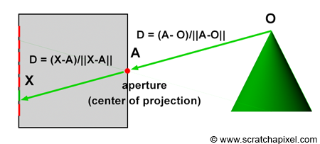
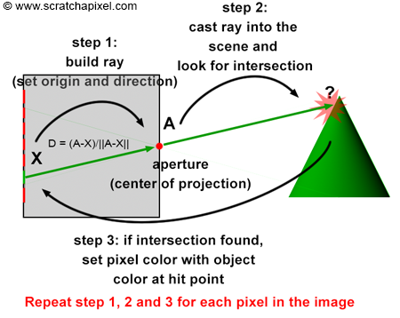
The operation of ray tracing, with respect to the camera model, is the opposite of how the rasterization algorithm functions. When a light ray, R, reflected off an object's surface, passes through the aperture of the pinhole camera and hits the image plane's surface, it strikes a particular pixel, X, as described earlier. In other words, each pixel, X, in an image corresponds to a light ray, R, with a given direction, D, and a given origin, O. It is important to note that knowing the ray's origin is not necessary to define its direction. The direction of the ray can be determined by tracing a line from O (the point where the ray is emitted) to the camera's aperture, A. It can also be defined by tracing a line from pixel X, where the ray intersects the camera's aperture, A (as shown in Figure 13). Therefore, if you can find the ray's direction, D, by tracing a line from X (the pixel) to A (the camera's aperture), then you can extend this ray into the scene to find O (the origin of the light ray), as shown in Figure 14. This principle, known as ray tracing or ray casting, allows us to produce an image by setting the pixel's colors to the colors of the light rays' respective points of origin. Due to the nature of the pinhole camera, each pixel in the image corresponds to one singular light ray, which we can construct by tracing a line from the pixel to the camera's aperture. We then cast this ray into the scene and set the pixel's color to the color of the object the ray intersects (if any—the ray might not intersect any geometry, in which case we set the pixel's color to black). This point of intersection corresponds to the point on the object's surface from which the light ray was reflected towards the eye.

Contrary to the rasterization algorithm, ray tracing is "image-centric". Instead of following the natural path of the light ray, from the object to the camera (as is done with rasterization), we follow the same path but in the opposite direction, from the camera to the object.

In our virtual camera model, rays are all emitted from the camera origin; thus, the aperture is reduced to a singular point (the center of projection), and the concept of aperture size in this model is nonexistent. Our CG camera model behaves as an ideal pinhole camera because we consider that a single ray only passes through the aperture (as opposed to a beam of light containing many rays, as with real pinhole cameras). This is, of course, impossible with a real pinhole camera, where diffraction occurs when the hole becomes too small. With such an ideal pinhole camera, we can create perfectly sharp images. Here is the complete algorithm in pseudo-code:

for (each pixel in the image) {
    // step 1
    build a camera ray: trace a line from the current pixel location to the camera's aperture;
    // step 2
    cast the ray into the scene;
    // step 3
    if (the ray intersects an object) {
        set the current pixel's color with the object's color at the intersection point;
    }
    else {
        set the current pixel's color to black;
    }
}

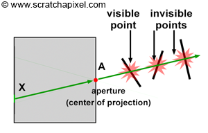
As explained in the first lesson, ray-tracing is a bit more complex because any camera ray can intersect several objects, as shown in Figure 15. Of all these points, the one visible to the camera is at the closest distance to the eye. If you are interested in a quick introduction to the ray-tracing algorithm, you can read the first lesson of this section or continue reading the lessons from this section devoted specifically to ray-tracing.

Advanced: You may have realized that several rays can strike the image at the same pixel location. This scenario is depicted in the adjacent image and occurs frequently in the real world because the surfaces from which the rays are reflected are continuous. In practice, we observe the projection of a continuous surface (the surface of an object) onto another continuous surface (the surface of a pixel). It's crucial to understand that a pixel in the physical world is not an ideal point but a surface that receives light reflected from another surface. A more accurate perception of this phenomenon, often adopted in computer graphics (CG), is viewing it as an "exchange" or transport of light energy between surfaces. For more information on this topic, refer to lessons in the Mathematics and Physics of Computer Graphics, specifically those covering the Mathematics of Shading and Monte Carlo Methods, as well as the lesson on Monte Carlo Ray Tracing and Path Tracing.

What's Next?

We are now prepared to implement a pinhole camera model with controls akin to those found in software like Maya. This will be accompanied by the source code for a program capable of producing images with output comparable to that of Maya.