Introduction to Acceleration Structures

Bounding Volume Hierarchy: BVH (part 1)

Introduction

In this chapter we will present and use a technique developed by the researchers Kay and Kajiya in 1986\. Other acceleration structures since this time have proven to be better than their technique, but their solution can help to lay down the principles upon which most acceleration structures are built. It is a very good starting point, and like with the Utah Teapot will give us an opportunity to introduce some new and interesting techniques which appear in many other computer graphics algorithms (such as the octree structure for instance). We highly recommend that you read their paper (check the references section at the end of this lesson).

Extent

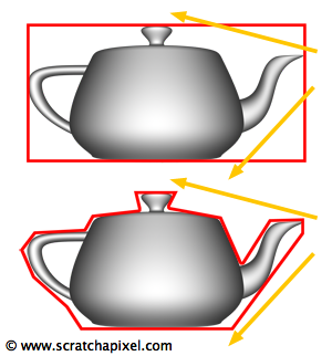
In the previous chapter, we intuitively showed that simple techniques such as ray tracing against bounding volumes could be used to accelerate ray tracing. As Kay and Kajiya point out in their paper, these techniques are only valid if ray tracing these bounding volumes or extents as they call them, is much faster than ray tracing the objects themselves. They also point out that if the extent fits an object loosely, then many of the rays intersecting this bounding volume are likely to actually miss the object inside. On the other hand, if the extent describes the object precisely, then all rays intersecting the extent will also intersect the object. Obviously, the bounding volume that fits this criteria is the object itself. A good choice for a bounding volume is therefore a shape that provides a good tradeoff between tightness (how close an extent fits the object) and speed (a complex bounding volume is more expensive to ray trace than a simple shape). This idea is illustrated in figure 1, where the box surrounding the teapot is faster to ray trace than the tighter bounding volume surrounding the teapot in the image below. However more rays intersecting this box will miss the teapot geometry than in the case of an extent fitting the model more closely. Shapes such as spheres and boxes give some pretty good results in most cases, but exploiting the idea of finding a good compromise between simplicity and speed, Kay and Kajiya propose to refine these simple shapes a step further.

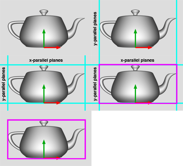
A bounding box can be seen as planes intersecting each other. To make this demonstration easier let's just consider the two-dimensional case. Let's imagine that we need to compute the bounding box of the teapot. Technically this can be seen as the intersection of two planes parallel to the y-axis with two planes parallel to the x-axis (figure 2). We now need to find a way of computing this planes? How do we do that? We have already presented the plane equation in the lesson 7 to compute the intersection of a ray with a box, as well in lesson 9, to compute the intersection of a ray with a triangle. Let's recall that the plane equation (in three dimensions this time) can be defined as:

where the terms A, B, C define the normal of the plane (a vector perpendicular to the plane) and \(d\) is the distance from the world origin to this plane along this vector. The terms x, y, z define the 3D cartesian coordinates of a point lying on the plane. This equation says that any point lying on the place whose coordinates are multiplied by the coordinates of the plane's normal, minus \(d\) is equal zero. This equation can also be used to project the vertices of the teapot onto a plane and find a value for \(d\). For a given point \(P_{(x, y, z)}\) and a given plane with normal \(N_{(x, y, z)}\) we can solve for \(d \):

We can re-write this equation as a more traditional point-matrix multiplication of the form (equation 1):

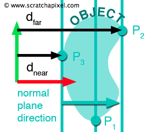
If we project a vertex \(P_{(x, y, z)}\) on the plane parallel to the y-axis with normal \(N_{(1, 0, 0)}\), \(d\) gives the distance along the x-axis from the origin to the plane parallel to the y-axis in which lies \(P_{(x, y, z)}\). If we repeat this process for all the vertices of the model, we can show that the point with the minimum \(d\) value and the point with the maximum \(d\) value, correspond to the object x-coordinate minimum and maximum extent respectively. These two values of \(d\), \(d^{near}\) and \(d^{far}\) describe two planes that bound the object (as showed in figure 3). We can implement this process with the following pseudocode:

// plane normal
vector N(1, 0, 0);
float Dnear = INFINITY;
float Dfar = -INFINITY;
for (each point in model) {
    // project point
    float D = N.x * P.x + N.y * P.y + N.z * P.z;
    Dnear = min(D, Dnear);
    Dfar = max(D, Dfar); 
}

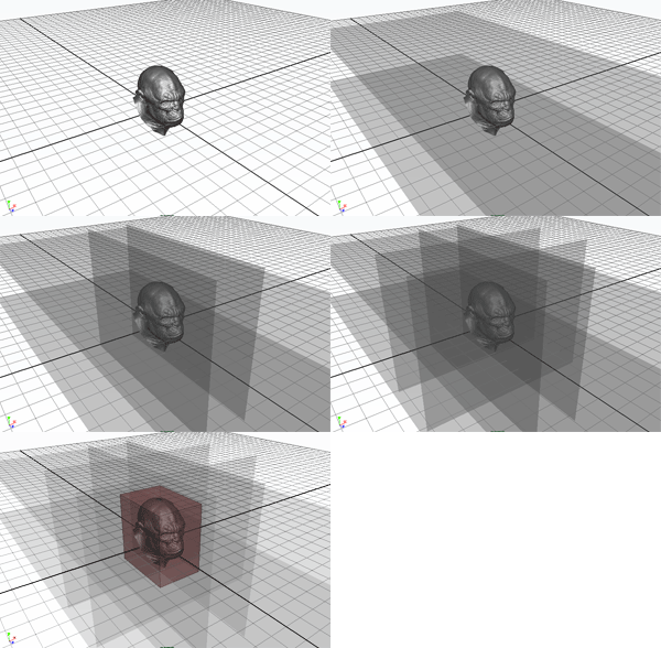
In their paper, Kay and Kajiya call the region in space between the two planes a slab and the normal vector defining the orientation of a slab is termed a plane-set normal. And as they observe:

Different choices of **plane-set normals** yield different bounding slabs for an object. The intersection of a set of bounding **slabs** yields a bounding volume. In order to create a closed bounding volume in 3-space, at least three bounding slabs must be involved, and they must be chosen so that the defining normal vectors span 3-space.

The simplest example of this principle is an axis-aligned bounding box (AABB) which is defined by three slabs respectively parallel to the xz-, yz- and xy-plane (figure 4). However, Kay and Kajiya propose to use not just three but seven slabs to get tighter bounding volumes. The plane-set normals of these slabs are chosen in advance and are independent of the objects to be bounded. To better visualise how this works let's go back again to the two-dimensional case. Let's imagine that the plane-set normals used to bound an object are:

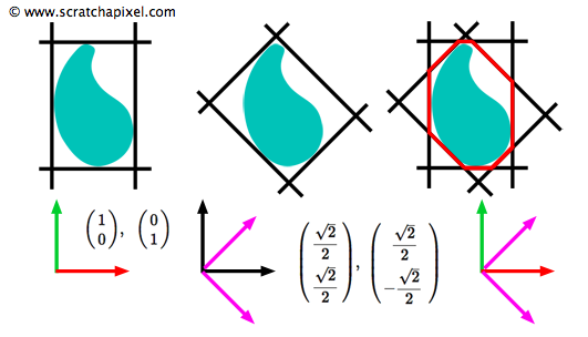
Figure 5 shows an object bounded by these pre-selected plane-set normals (this is a reproduction of figure 3 in Kay and Kajiya's paper).

As you can see, the resulting bounding box fits the object better than a simple bounding box. For the three-dimensional case, they use seven plane-set normals:

The first three plane-set normals define an axis-aligned bounding box and the last four plane-set normals, define an eight sided parallelepiped. To Build a bounding volume of an object, we simply find the minimum and maximum value of \(d\) for each slab by projecting the vertices of the model on the seven plane-set normals.

Ray-Volume Intersection

Next, we need to write some code to ray trace the volumes. The principle is very similar to that of the ray-box intersection. A slab is defined by two planes parallel to each other, and if the ray is not parallel to these planes, it will intersect them both yielding two values, \(t_{min}\) and \(t_{far}\). To compute the intersection distance \(t\) we simply substitute the ray equation \(O + Rt = 0\) into the plane equation \(Ax + By + Cz - d = N_i \cdot P_{x,y,z} - d = 0\) yielding (equation 2):

where \(N_i\) is one of the seven plane-set normals, \(O\) and \(R\) are respectively the origin and direction of the ray and \(d\) the distance from the world origin to the plane with normal \(N_i\) in which lies the intersection point \(P_{x,y,z}\). The two terms \(N_i \cdot O\) and \(N_i \cdot R\) can be re-used to compute the intersection distance \(t\) between the ray and the two planes. Substituting the pre-computed values of \(d\) (\(d_{near}\) and \(d_{far}\)) for the tested slab yields a value \(t\) for each plane.

// computing intersection of a given ray with slab
float NdotO = N . O;
float NdotR = N . R;
float tNear = (dNear - NdotO) / NdotR;
float tFar = (dFar - NdotO) / NdotR;

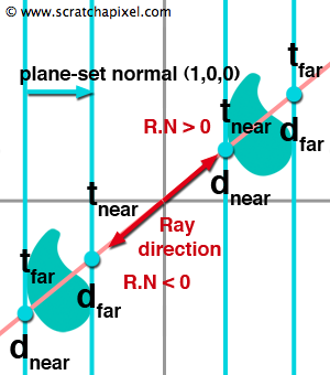
Like with the ray tracing of boxes, care must be taken when the denominator \(N_i \cdot R\) is close to zero. Furthermore, when the denominator is lower than zero we also need to swap \(d_{near}\) and \(d_{far}\) (see figure 6). As for the ray-box intersection (see lesson 7 for more information on the algorithm), this test is performed for each slab enclosing the object. Of all the computed \(t_{near}\) values we will keep the largest one, and of all the computed \(t_{far}\) values, we will keep the smallest one. An intersection with the volume occurs if the final \(t_{far}\) value is greater than the \(t_{near}\) value. If the ray intersects the volume, the \(t\) values indicate the position of these intersections along the ray. The resulting interval (defined by \(t_{near}\) and \(t_{far}\)) is useful as an estimate of the position of the object along the ray. Let's now try to put what we learned into practice.

Source Code

The following C++ code implements the method described in this chapter. A BVH class is derived from the base AccelerationStructure class. We create a structure called Extents in this class which holds the values of \(d_{near}\) and \(d_{far}\) for all seven pre-defined plane-set normals (lines 7-11).

class BVH : public AccelerationStructure
{
    static const uint8_t kNumPlaneSetNormals = 7;
    static const Vec3f planeSetNormals[kNumPlaneSetNormals];
    struct Extents
    {
        Extents()
        {
            for (uint8_t i = 0; i < kNumPlaneSetNormals; ++i)
                d[i][0] = kInfinity, d[i][1] = -kInfinity;
        }
        bool intersect(const Ray<float> &ray, float &tNear, float &tFar, uint8_t &planeIndex);
        float d[kNumPlaneSetNormals][2];
    };
    Extents *extents;
public:
    BVH(const RenderContext *rcx);
    const Object* intersect(const Ray<float> &ray, IsectData &isectData) const;
    ~BVH();
};

In the constructor of the class we allocate an array of extents to store the bounding volume data for all the objects in the scene (line 3). Then we loop over all the objects and call the method computeBounds from the Object class to compute the values dNear and dFar for each slab enclosing the object (lines 4-8). In the following code snippet we only show this function for the PolygonMesh class. We loop over all the vertices of the mesh and project them on the current plane (lines 27-31). This conclude the work done in the class constructor.

BVH::BVH(const RenderContext *rcx) : AccelerationStructure(rcx), extents(NULL) 
{ 
    extents = new Extents[rcx->objects.size()]; 
    for (uint32_t i = 0; i < rcx->objects.size(); ++i) { 
        for (uint8_t j = 0; j < kNumPlaneSetNormals; ++j) { 
            rcx->objects[i]->computeBounds(planeSetNormals[j], extents[i].d[j][0], extents[i].d[j][1]); 
        } 
    } 
} 

const Vec3f BVH::planeSetNormals[BVH::kNumPlaneSetNormals] = { 
    Vec3f(1, 0, 0), 
    Vec3f(0, 1, 0), 
    Vec3f(0, 0, 1), 
    Vec3f( sqrtf(3) / 3.f,  sqrtf(3) / 3.f, sqrtf(3) / 3.f), 
    Vec3f(-sqrtf(3) / 3.f,  sqrtf(3) / 3.f, sqrtf(3) / 3.f), 
    Vec3f(-sqrtf(3) / 3.f, -sqrtf(3) / 3.f, sqrtf(3) / 3.f), 
    Vec3f( sqrtf(3) / 3.f, -sqrtf(3) / 3.f, sqrtf(3) / 3.f) }; 
} 

class PolygonMesh : public Object 
{ 
    ... 
    void computeBounds(const Vec3f &planeNormal, float &dnear, float &dfar) const 
	{ 
        float d; 
        for (uint32_t i = 0; i < maxVertIndex; ++i) { 
            d = dot(planeNormal, P[i]); 
            if (d < dnear) dnear = d; 
            if (d > dfar) dfar = d; 
        } 
    } 
    ... 
}; 

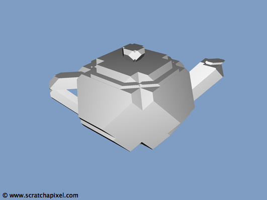
Once the render function is called, rather than intersecting each object of the scene, we call the intersection method from the BVH class. First the ray is tested against all the bounding volumes of all the objects from the scene. To do so, we call the intersect method from the Extent structure with the volume data of the current tested object (line 24). This method simply computes the intersection of the current ray with each of the seven slabs enclosing the object and tracks the greatest of the dNear values and the smallest of the computed dFar values. If dFar is greater than dFar, then an intersection with the bounding volume occurs and the function returns true. In the following version of the code, if the ray intersects the volume we set the member variable N from the IsectData structure with the normal of the intersected plane. The result of the dot product of this vector N with the ray direction is used to set the color of the current pixel. The resulting image can be seen in figure 7. This helps to visualise the bounding volumes being intersected and surrounding the objects.

inline bool BVH::Extents::intersect(
	const Ray<float> &ray,
    float *precomputedNumerator, float
	*precomputeDenominator,
	float &tNear, float &tFar, uint8_t
	&planeIndex)
{
	for (uint8_t i = 0; i < kNumPlaneSetNormals; ++i) {
        float tn = (d[i][0] - precomputedNumerator[i]) / precomputeDenominator[i];
        float tf = (d[i][1] - precomputedNumerator[i]) / precomputeDenominator[i];
        if (precomputeDenominator[i] < 0) std::swap(tn, tf);
        if (tn > tNear) tNear = tn, planeIndex = i;
        if (tf < tFar) tFar = tf;
        if (tNear > tFar) return false;
    }
 
    return true;
}

const Object* BVH::intersect(const Ray<float> &ray, IsectData &isectData) const
{
	float tClosest = ray.tmax;
    Object *hitObject = NULL;
    float precomputedNumerator[BVH::kNumPlaneSetNormals], precomputeDenominator[BVH::kNumPlaneSetNormals];
    for (uint8_t i = 0; i < kNumPlaneSetNormals; ++i) {
        precomputedNumerator[i] = dot(planeSetNormals[i], ray.orig);
        precomputeDenominator[i] = dot(planeSetNormals[i], ray.dir);;
    }
    for (uint32_t i = 0; i < rc->objects.size(); ++i) {
        __sync_fetch_and_add(&numRayVolumeTests, 1);
        float tNear = -kInfinity, tFar = kInfinity;
        uint8_t planeIndex;
        if (extents[i].intersect(ray, precomputedNumerator, precomputeDenominator, tNear, tFar, planeIndex)) {
            if (tNear < tClosest)
                tClosest = tNear, isectData.N = planeSetNormals[planeIndex], hitObject = rc->objects[i];
        }
    }
 
    return hitObject;
}

But in the following and final version of the intersect method, if the bounding volume is intersected, we then test if there is an intersection between the ray and the object (or objects if it is a grid of triangles for example) enclosed by the volume. When the test is successful, we update tClosest if the intersection distance is the smallest we have found so far and keep a pointer to the intersected object.

int main(int argc, char **argv)
{
    clock_t timeStart = clock();
    ...
    rc->accelStruct = new BVH(rc);//AccelerationStructure(rc);
    render(rc, filename);
    ...
    printf("Render time                                 : %04.2f (sec)\n", (float)(timeEnd - timeStart) / CLOCKS_PER_SEC);
    printf("Total number of triangles                   : %d\n", totalNumTris);
    printf("Total number of primary rays                : %llu\n", numPrimaryRays);
    printf("Total number of ray-triangles tests         : %llu\n", lrt::numRayTrianglesTests);
    printf("Total number of ray-triangles intersections : %llu\n", lrt::numRayTrianglesIsect);
    printf("Total number of ray-volume tests            : %llu\n", lrt::numRayBoxTests);
    return 0;
}

Finally, if we compile and run the program using our new acceleration structure we get the following the statistics:

Render time                                 : 2.92 (sec)
Total number of triangles                   : 16384
Total number of primary rays                : 307200
Total number of ray-triangles tests         : 80998400
Total number of ray-triangles intersections : 111889
Total number of ray-volume tests            : 9830400

This technique is 1.34 times faster than the method from the previous chapter. It might not seem much but a few saved seconds on a simple scene can turn into hours on a complex one.

What's Next?

Even though we have improved the results from chapter 2 this technique still suffers from the fact that the rendering time is proportional to the number of objects in the scene. To improve the performance of this method a step further, Kay and Kajiya suggest to use a hierarchy of volumes. Quoting the authors of the paper again:

For each such node we compute a bounding volume. Then if a ray misses the bounding volume at a given node in the hierarchy, we can reject that node's entire subtree from further consideration. Using a hierarchy causes the cost of computing an image to behave logarithmically in the number of objects in the scene.

We will implement this idea in the next chapter.