Grid
Reading time: 37 mins.In this chapter we will describe a technique proposed by Akira Fujimoto in 1986 (in a paper entitled "ARTS: Accelerated Ray Tracing Systems"). The idea is to subdivide space in sub-regions and as the ray passes through these sub-regions, check if they contain geometry that we should ray-trace against (this algorithm belongs to the category of methods called spatial division also called spatial coherence or space tracing). Rather than checking rays against all objects in the scene or against bounded volume approximations to the objects in the scene, these methods are used to determine if the region through which the ray is passing, is occupied by objects. This idea is illustrated in the following figure.
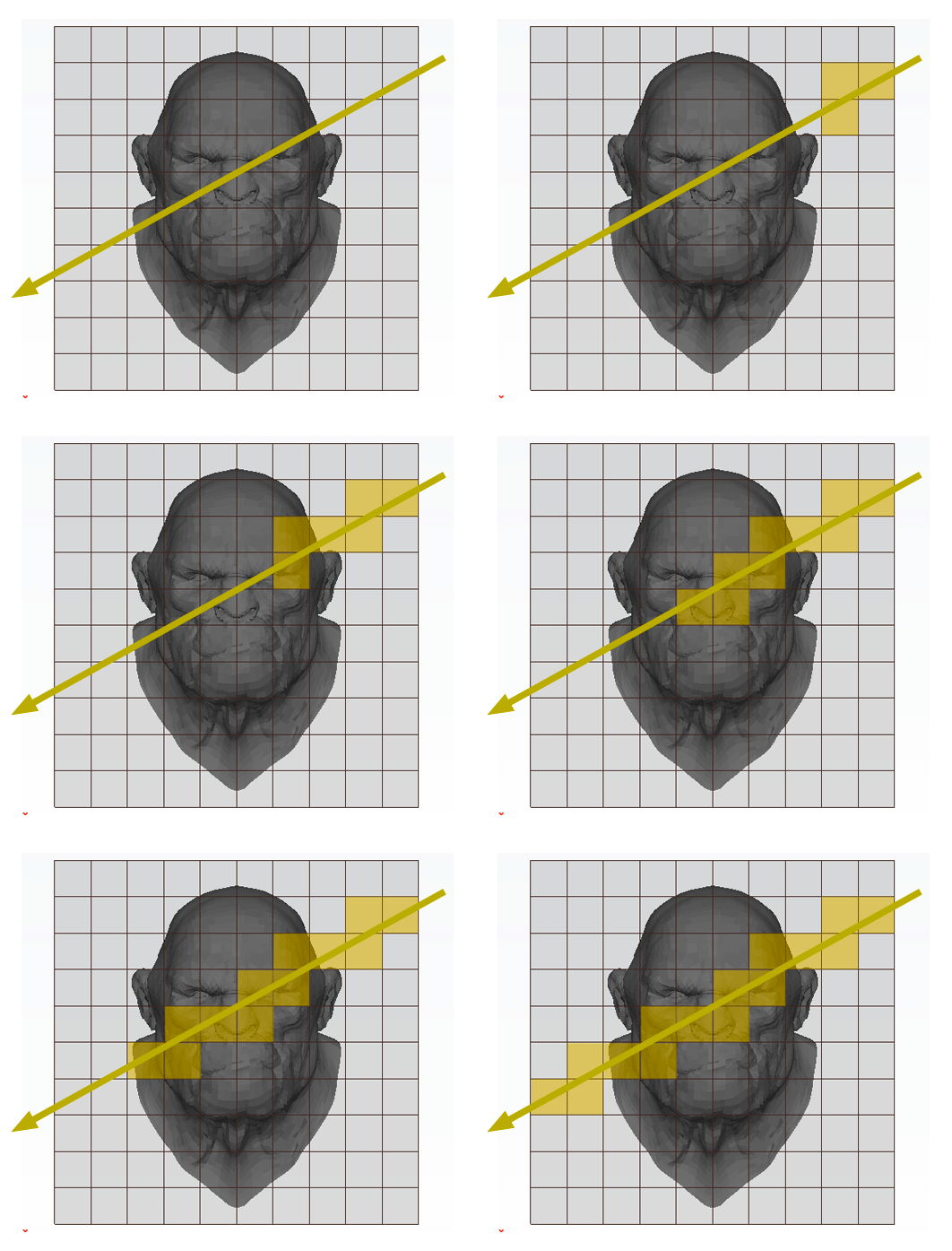
The principle is very simple. We subdivide the region of space containing the object into a regular 3D grid (in figure 1, the technique is illustrated in 2D). We will explain how we chose the size and the resolution of the grid later. Triangles of the models are then inserted in the grid's cells they overlap. Some cells will be empty but others will contain a subset of the models' geometry (this can be seen as breaking the models into regular chunks). We will look at the details of this step later. This concludes the pre-processing part of the algorithm. Testing if a ray intersects the models' geometry is simple. We traverse the grid cell by cell following the ray's direction. If the current cell is occupied by some geometry then we check if the ray intersects this geometry. If it does, we can stop traversing the grid, otherwise, we move to the next cell pierced by the ray. This process is repeated until the ray hits an object or until the ray leaves the grid. For reference, this grid was termed by Fujimoto a Spatially Enumerated Auxiliary Data Structure (and was given the acronym SEADS).
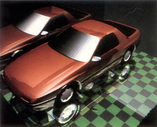
The grid approach is good because it automatically subdivides the objects into smaller chunks which are faster to test than the entire models. Furthermore, if we were to represent the ray's traversal process in terms of parametric distance \(t\), we could say that \(t\) increases monotonically as we go from one cell to another. Finally, Fujimoto developed an algorithm called a 3D-Digital Differential Analyser (or DDA) which makes the traversal of the grid simple and fast. First, we will study this algorithm, then we will explain how the geometry of the models is inserted into the grid's cells. The following image was produced by Fujimito and his team using their algorithm.
3D-Digital Differential Analyser
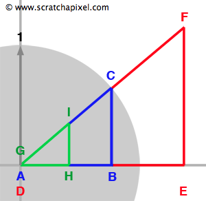
To better understand how the DDA algorithm works, let's first review some facts regarding similar triangles. Similar triangles are triangles that have two identical angles (which means that all the angles are the same).
We have represented three such triangles in Figure 2. They can also be seen as magnified or reduced copies of each other. One important property of such triangles is that the ratio between their side is identical. For example we can write (equation 1):
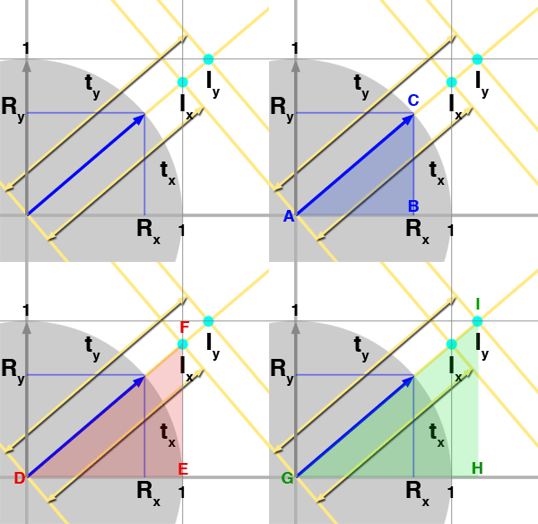
$${ {{AB} \over {DE}} = {{BC} \over {EF}} = {{AC} \over {DF}}}$$Now that we have reviewed this fact let's talk about the problem we are trying to solve. We need to find all the cells from a grid that a ray is intersecting with. What we know about the ray is its origin \(O\) and direction \(R\). To simplify the demonstration, we will be working in 2D (before generalizing to 3D) and assume that the grid's cell has size 1\. We have illustrated the problem in figure 3 with a ray starting at the origin and which direction is indicated by the blue arrow. As you can see, the ray passes through another cell as soon as it crosses a line in either the vertical (at \(I_x\)) or horizontal direction (at \(I_y\)). We also know that the parametric value \(t\) indicates the distance from the ray's origin to any point on the ray (the ray equation is \(P = O + Rt\)). The question is: can we compute values of \(t\) for which the ray intersects the cells' vertical and horizontal boundaries, which in this example, are noted \(t_x\) and \(t_y\) for the first two intersections? The answer to this is simple. As shown in figure 3, using the ray direction (the blue arrow) we can define the right angle triangle \(\Delta ABC\). Note that because the ray direction is normalized, \(||AC||\) equals one (the length of the vector AC). We also know Rx and Ry which corresponds to B and C respectively. What we are trying to compute is \(t_x\) which is also equal in our figure to the hypotenuse of the right triangle \(\Delta DEF\). We also know about \(\Delta DEF\) that \(||DE||\) equals one. The triangles \(\Delta ABC\) and \(\Delta DEF\) are similar therefore we can write (using equation 1):
$${{AB} \over {DE}} = {{AC} \over {DF}} = {R_x \over 1} = {1 \over t_x}$$And thus:
$$t_x = { 1 \over R_x } $$We can do the same reasoning for \(t_y\) however this time we will be using the opposite side of the triangle \(\Delta GHI\):
$${{BC} \over {HI}} = {{AC} \over {GI}} = {R_y \over 1} = {1 \over t_y}$$Therefore:
$$t_y = { 1 \over R_y } $$And not surprisingly, in 3D:
$$t_z = { 1 \over R_z }$$We can now compute \(t_x\), \(t_y\) (and \(t_z\)).
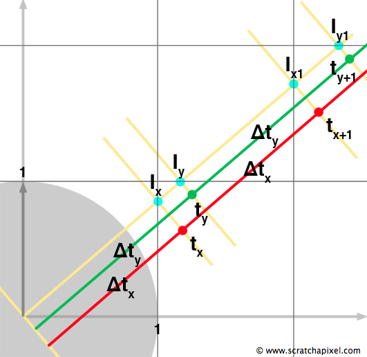
Figure 4 is the same as figure 3 except that we have now represented the next two intersections along the ray. As you can visually see, the distance along the ray from the intersection point \(I_x\) to the next intersection point \(I_{x1}\), is the same as the distance from the origin to \(I_x\). The same remark applies to \(I_y\) and \(I_{y1}\): the distance between \(I_y\) and \(I_{y1}\) is the same as the distance from the origin of the ray to \(I_y\). If \(t_x\) and \(t_y\) are the parametric distances along the ray to the current intersection point along either the x-axis and y-axis respectively, and \(\Delta t_x\) and \(\Delta t_y\) are the distances between two consecutive intersection points along either the x- and y-axis respectively, then the next intersection point along either one of these axes can be computed using the following formula:
$$t_{x+1} = t_x + {\Delta t_x} \text{ and } t_{y+1} = t_y + {\Delta t_y}$$The goal of the algorithm is to find each cell the ray is passing through. We can easily do that if we can compute the intersection points between the ray and the cells' boundaries (define in our example as the lines along the x- and y-axis). At the beginning of the process, we initialize \(t\), \(t_x\) and \(t_y\), and calculate \(\Delta_x\) and \(\Delta_y\):
$$t = 0, t_x = 0, t_y = 0, \Delta t_x = { 1 \over R_x}, \Delta t_y = { 1 \over R_y }$$To compute the next intersection point along the x- and y-axis we do:
$$ \begin{array}{l} t_x += \Delta t_x,\\ t_y += \Delta t_y \end{array} $$This gives us the distances to the next two intersection points with a cell, the next intersection along the x-axis and the next intersection along the y-axis, but which one of the boundaries does the ray intersect first? The answer to this is simple, it is the boundary for which the distance is the closest. In other words, if \(t_x < t_y\) the ray intersects the cell along the x-axis otherwise it intersects the ray along the y-axis. If the ray intersects the cell along the x-axis then we update \(t_x\) with the new distance to the next intersection point along the x-axis:
$$t_x += \Delta t_x$$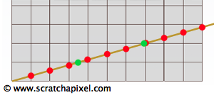
And we repeat the question. Which one of \(t_x\) or \(t_y\) is the smallest. If \(t_x\) is the smallest then we cross another cell in the x-axis direction otherwise we cross a new cell in the y-direction. With the ray from Figure 4, we would get the following sequence: cross x, cross y, cross x, cross y. However, in the example on the right (figure 5) the sequence of intersections would be x, x, x, y, x, x, x, y, x, x, x, x. We can put all the things we have learned so far and write a very simple 2D DDA algorithm in pseudocode:
Vec2f RayDirection = { ..., ... }; // assumed normalized
Vec2f deltaT = { 1 / RayDirection[0], 1 / RayDirection[1] };
foat t_x = deltaT[0], t_y = deltaT[1], t = 0;
while (1) {
	if (t_x < t_y) {
        t = t_x; // current t, next intersection with cell along ray
        t_x += deltaT[0]; // increment, next crossing along x
    }
    else {
        t = t_y;
        t_y += deltaT[1]; // increment, next crossing along y
    }
    // if some condition is met break from the loop
    if (...) break;
}
That's in essence how the DDA algorithm works which can be used for many things. However, to be useful we need to keep track of the cells the ray is traversing so that later, we can test for an intersection between the ray and the geometry contained by the cell. This is simple. We know we start from the cell (0, 0) and each time we cross a vertical line we increment the cell index in x, and each time we cross a horizontal line we increment the cell index in y. The sequence of cells traversed in Figure 5 is: (0,0), (1,0), (2,0), (3,0), (3,1), (4,1), (5,1), (6,1), (6,2), etc. Let's update our pseudocode:
Vec2f rayDirection = { ..., ... }; // assumed normalized
Vec2f deltaT = { 1 / rayDirection[0], 1 / rayDirection[1] };
float t_x = deltaT[0], t_y = deltaT[1], t = 0;
Vec2i cellIndex = {0, 0};
while (1) {
    if (t_x < t_y) {
        t = t_x; // current t, next intersection with cell along ray
        t_x += deltaT[0]; // increment, next crossing along x
        cellIndex[0] += 1;
    }
    else {
        t = t_y;
        t_y += deltaT[1]; // increment, next crossing along y
        cellIndex[1] += 1;
    }
    // if some condition is met break from the loop
    if (...) break;
}
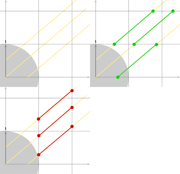
To make the algorithm robust though we need to take into consideration a few more problems. First, the ray doesn't necessarily start at the origin, the ray direction is not always positive (e.g. \(Rx > 0\) and \(Ry > 0\)), the grid is not always a unit grid (where the cell size equals one) and finally, we need to stop the traversal process when the ray exits the grid.
Let's see what happens when the ray doesn't start at the origin. Note that changing the ray position in x or y doesn't change the value of \(\Delta_x\) or \(\Delta_y\) (figure 6). The part of the algorithm computing these values is therefore the same. As you can see in figure 7, the only thing that changes is the initial value of \(t_x\) and \(t_y\). They now need to be computed using the following formula:
$$ \begin{array}{l} t_{x0} = \dfrac{1 - O_x}{R_x },\\ t_{y0} = \dfrac{1 - O_y}{R_y } \end{array} $$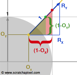
The technique used with similar triangles before can be used again. Only now DE from figure 3 is replaced with \((1-Ox)\) and HI is replaced with \((1-Oy)\).
The second problem we need to account for is the size of the cell which is not necessarily one. The overall size of the grid used as an acceleration structure is the same as the scene's overall bounding box. We will then divide this bounding box into a certain number of cells (how we find this number will be discussed later). Thus, in almost all cases not only the size of the cell is not one, but the cells are not cubes either. The values in each dimension are usually different from each other. Figure 8 illustrates this situation. The size of the cell is larger than one in x and smaller than one in y. However, if we draw the triangles \(\Delta ABC\) and \(\Delta DEF\) we see that we can use the similar triangle technique again to compute \(\Delta t_x\):
$$ \begin{array}{l} \dfrac{AB}{DE} = \dfrac{AC}{DF} = \dfrac{R_x}{cell\:size_x} = \dfrac{1}{\Delta t_x}\\ \Delta t_x = \dfrac{cell\:size_x}{R_x} \end{array} $$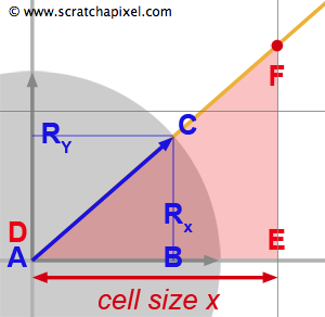
The same reasoning can be used to find \(\Delta t_y\). We also need to take into account the cell size when we compute initial values for \(t_x\) and \(t_y\):
$$ \begin{array} {l} t_{x0} = \dfrac{{cell\:size_x} - O_x}{R_x }\\ t_{y0} = \dfrac{{cell\:size_y } - O_y}{R_y } \end{array} $$Let's now see what happens when the ray direction is not positive. Imagine for example that \(R_x\) and \(R_y\) are lower than zero. The values for \(\Delta t_x\) and \(\Delta t_y\) would be negative therefore we need to invert their sign (these values are used to move along the ray in the ray direction therefore they have to be positive):
$$ \begin{array}{l} \Delta t_x = - {\dfrac{cell\:size_x }{R_x}} \text{, if } R_x < 0 \\ \Delta t_y = - {\dfrac{cell\:size_y }{R_y}} \text{, if } R_y < 0 \end{array} $$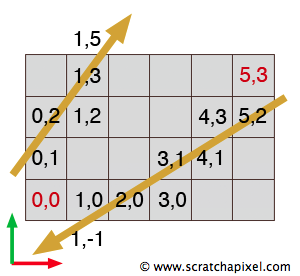
Furthermore each time we cross the boundary of a cell along the x- or y-axis, we need to decrement the cell index (instead of incrementing it). This is illustrated in figure 9.
The last problem to solve is to stop walking through the grid when the ray leaves the grid. This is simple. We know the dimension of the grid and we also keep track of the cell position (cell index) as we walk through the cells. Therefore as soon as one of the indexes in either x or y is greater than the grid dimension we can break from the loop. Here again, we need to pay attention to the direction of the ray. If the ray goes backward (has a negative direction in either x or y) the ray leaves the grid when we reach a cell whose index is lower than zero in either x or y (figure 9).
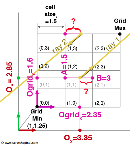
Finally we need to make a correction to the way we compute the initial values for \(t_{x0}\) and \(t_{y0}\). As you can see in figure 10, the ray doesn't necessarily start in the lower left cell of the grid. First, we need to convert the position of the origin of the ray in regards to the lower left corner of the grid which we can easily do by subtracting the grid minimum extent to the ray's origin. What we need at the end is a value for B so that we can compute the distance represented by an interrogation mark in Figure 10 (ray 1). The distance can be calculated by subtracting the origin of the ray in the relation to the origin of the grid (Ogrid in the figure) to B. The question is how do we compute B? We first "normalized" Ogrid by dividing it by the cell's dimensions. The resulting value corresponds to the position of the origin of the ray in terms of the number of cells. In our example the value 2.35 (Ogrid's x coordinate value) is divided by 1.5 (the dimension of the cell in x) which is equal to 1.567. If we take this value's nearest integer down, we effectively get the index of the cell in x in which the ray originates (1). Adding one to this value (1+1=2) and multiplying again by the cell size in x (2 * 1.5), gives the position for B (3). Here is the formula to compute \(t_{x0}\) and \(t_{y0}\) for an arbitrary ray origin:
$$ \begin{array}{l} Ogrid = O - GridMin\\ Ocell = \dfrac{Ogrid}{cell\:size}\\ t_{x0} = \dfrac{(floor(Ocell_x) + 1) * cell\:size_x - Ogrid_x}{R_x} \\ t_{y0} = \dfrac{(floor(Ocell_y) + 1) * cell\:size_y - Ogrid_y}{R_y} \end{array} $$However we need to be careful about the ray direction again. If the ray direction is negative along the x- or y-axis, the formula is slightly different. We have illustrated this situation in figure 10 with a second ray (ray 2) in which direction is negative. The distance represented by the interrogation mark can be computed by subtracting A from Ogrid rather than Ogrid from B as with the first example. However because the ray direction is negative and we want \(t_{x0}\) and \(t_{y0}\) to be positive, we will subtract Ogrid from A which result is negative (rather than A from Ogrid which result is positive). The two negative numbers on the numerator and denominator cancel out to form a positive number:
$$ \begin{array}{l} t_{x0} = \dfrac{floor(Ocell_x) * cell\:size_x - Ogrid_x}{R_x} \\ t_{y0} = \dfrac{floor(Ocell_y) * cell\:size_y - Ogrid_y}{R_y } \end{array} $$Here is a more solid version of the DDA algorithm in pseudocode:
Vec2f rayDirection = { ..., ... }; // assumed normalized
Vec2f rayOrigin = { ..., ... };
Vec2f gridResolution = { ..., ... };
Vec2f cellDimension = (gridMax - gridMin) / gridResolution;
Vec2f deltaT, nextCrossingT;
Vec2f rayOrigGrid = rayOrigin - gridMin;
if (rayDirection[0] < 0) {
    deltaT[0] = -gridDimension[0] / RayDirection[0]
    t_x = (floor(rayOrigGrid[0] / cellDimension[0]) * cellDimension[0]
        - rayOrigGrid[0]) / rayDirection[0];
}
else {
    deltaT[0] = gridDimension[0] / RayDirection[0];
    t_x = ((floor(rayOrigGrid[0] / cellDimension[0]) + 1) * cellDimension[0]
        - rayOrigGrid[0]) / rayDirection[0];
}
if (rayDirection[1] < 0) {
    deltaT[1] = -gridDimension[1] / RayDirection[1]
    t_y = (floor(rayOrigGrid[1] / cellDimension[1]) * cellDimension[1]
        - rayOrigGrid[1]) / rayDirection[1];
}
else {
    deltaT[1] = gridDimension[1] / RayDirection[1]
    t_y = ((floor(rayOrigGrid[1] / cellDimension[1]) + 1) * cellDimension[1]
        - rayOrigGrid[1]) / rayDirection[1];
}
float t = 0;
Vec2i cellIndex = { .., ... }; // origin of the ray (cell index)
while (1) {
    if (t_x < t_y) {
        t = t_x; // current t, next intersection with cell along ray
        t_x += deltaT[0]; // increment, next crossing along x
        if (rayDirection[0] < 0)
            cellIndex[0] -= 1;
        else
            cellIndex[0] += 1;
    }
    else {
        t = t_y;
        t_y += deltaT[1]; // increment, next crossing along y
        if (rayDirection[1] < 0)
            cellIndex[1] -= 1;
        else
            cellIndex[1] += 1;
    }
	// if some condition is met break from the loop
    if (cellIndex[0] < 0 || cellIndex[1] < 0 ||
        cellIndex[0] > gridDimension[0] - 1 || cellIndex[1] > gridDimension[1] - 1)
        break;
}
Creating the Grid and Inserting the Object
In the previous section we have explained how the grid can be traversed efficiently using the DDA algorithm. We will now explain how we create the grid and particularly insert the geometry in the grid's cells. The use of a grid is not limited to triangulated objects however this is the only example we will show in this lesson (hence the advantage of converting different types of geometry to the same triangulated mesh representation). First, we need to compute an overall bounding box of the grid, the same as the scene bounding box. We can simply loop over all the objects of the scene and merge their bounding boxes. Once we have the size of the grid, the next task consists of choosing its resolution (the number of cells in each dimension). Unfortunately, there is no formula to compute a resolution that could be proven to be optimum for all the scenes or even a given scene. Some metrics have been developed but most of the time still relies on a user-defined parameter to fine-tweak the performance of the scheme. This is potentially a disadvantage of the grid method. The method used to compute the grid resolution is most of the time based on a metric proposed by Cleary in 1983 in a paper entitled "A Parallel Ray Tracing Computer". The formula is (equation 1):
$$ \begin{array}{l} N_x = d_x \sqrt[3]{\dfrac{\lambda N}{V}}\\ N_y = d_y \sqrt[3]{\dfrac{\lambda N}{V}} \\ N_z = d_z \sqrt[3]{\dfrac{\lambda N}{V}} \end{array} $$where \(N_x\), \(N_y\) and \(N_z\) define the grid resolution in each dimension, \(d_x\), \(d_y\) and \(d_z\) define the size of the grid (the scene bounding box), \(N\) is the number of triangles contained in the grid and \(V\) is the volume of the scene bounding box. Without getting into too many details, you can see that this formula tries to establish some relation between the dimension of the scene, the number of primitives it contains, and the overall volume of the scene. The parameter \(\lambda\) is a user-defined parameter which allows to fine tweak the performance of the algorithm. If the resolution is too high, the time spent traversing the scene using the 3D-DDA algorithm outweighs the benefit of using the acceleration structure. On the other hand if the resolution is too low the cell contains many triangles and the time spent intersecting each triangle contained in the cells doesn't make the grid a much better method than simpler acceleration methods (such as the bounding box for instance). It has been shown that the grid acceleration structure gives optimum results for values of \(\lambda\) between 3 and 5 ("Ray Tracing Animated Scenes using Coherent Grid Traversal", Wald et al. 2006).
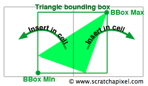
Now that we have both the size and the resolution of the grid we can insert the triangles into the cells. We will loop over all the triangulated objects of the scene, and for each object, loop over all the triangles from the current mesh. The bounding box of each triangle is first computed and then converted to cell coordinates by dividing the extents of the bounding box over the cell size:
$$ \begin{array}{l} cell\:size = \frac{grid\:size}{grid\:resolution}\ min\:cell=\frac{triangle\:BBox\:min}{cell\:size}\\ max\:cell=\frac{triangle\:BBox\:max}{cell\:size} \end{array} $$The result represents a box that overlaps the cells from the grid that the triangle potentially overlaps (as shown in figure 11). The next task consists of looping over the cells overlapped by this box and inserting the triangle into these cells.
for (int z = cellMin.z; z <= cellmax.z; ++z)
    for (int y = cellMin.y; y <= cellmax.y; ++y)
        for (int x = cellMin.x; x <= cellmax.x; ++x)
            cell[x][y][z].insert(triangle);
The difficulty here (from a coding point of view more than from an algorithmic point of view) is to avoid duplicating the information about the triangle which is already stored in the mesh. If we had to store the triangle as three vertices in each of the overlapped cells, in the best scenario, we would double the memory used to store the geometry data. All we need to access the triangle data is a pointer to the mesh the triangle belongs to, and an offset in the vertex array data which can be used to retrieve the three vertices making up the triangle. This referencing mechanism is described in more detail in the source code section. Once all the triangles of all the meshes have been inserted into the cells, the grid creation process is finished (note that a cell can contain more than one triangle). Implementation details can be found in the source code section.
Intersecting the Grid

Finally we are left with describing the ray-grid intersection process. Before traversing the grid we can first check if the ray hits the grid at all, which can be done with a simple ray-box intersection test. If the ray intersects the grid we can then compute the coordinates of the cell where the ray enters the grid (figure 12). Once we know the start position of the ray in the grid (which requires converting the hit point or the ray's origin if the ray is inside the grid to cell coordinates), we simply use the DDA algorithm to efficiently walk through the grid in the direction of the ray and test for an intersection with the geometry contained by every cell the ray passes through.
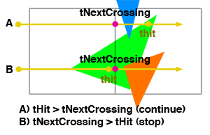
In Figure 13 we have shown that a ray can traverse cells that contain the same triangle (green). This triangle might be intersected several times which is a potential problem in terms of efficiency but we will talk about that later. Ray A intersects the green triangle but the intersection distance is further away than the intersection distance with the next crossed cell (tNextCrossing). Even though we have an intersection, it is not safe to stop the traversal at this point (it would if we were only computing shadow rays but for primary rays, we need to find the visible object. This will become clear in the lessons dedicated to shading). The next cell (cell 2) contains a blue triangle which is intersected by ray A before the green triangle. The visible object is the blue triangle, not the green one, and stopping the traversal at cell 1 would not return the visible geometry for this ray. For ray B, the intersection distance with the green triangle is smaller than the distance to the next cell. In that case, no over triangle can be closer to the ray than the green triangle, and we can stop the grid traversal at cell 1.
bool intersect = false;
float tHit;
while (1) {
    intersect |= cell[cellIndex[0]][cellIndex[1]]->intersect(ray, tHit);
    if (t_x < t_y) {
        tNextCrossing = t_x; // current t, next intersection with cell along ray
        t_x += deltaT[0]; // increment, next crossing along x
        if (rayDirection[0] < 0)
            cellIndex[0] -= 1;
        else
            cellIndex[0] += 1;
    }
    else {
        tNextCrossing = t_y;
        t_y += deltaT[1]; // increment, next crossing along y
        if (rayDirection[1] < 0)
            cellIndex[1] -= 1;
        else
            cellIndex[1] += 1;
    }
    // if we have intersected geometry and tHit < tNextCrossing break
    if (intersect && tHit < tNextCrossing) break;
    // if some condition is met break from the loop
    if (cellIndex[0] < 0 || cellIndex[1] < 0 ||
        cellIndex[0] > gridDimension[0] - 1 || cellIndex[1] > gridDimension[1] - 1)
        break;
}
Mail Boxing
We mentioned before that a triangle may be inserted in more than one cell when its bounding box straddles the boundaries of a cell. Figure 12 shows what can happen in this case. The green triangle is tested for an intersection with ray A twice (when a ray traverses one cell there is a high probability it will traverse the neighboring cells as well which most likely reference the same geometry). The goal of the acceleration structure is to reduce as much as possible the number of intersection tests and having to compute the intersection of a ray with the same triangle multiple times can reduce the performance of the grid acceleration method. One possible solution to this problem is to use a technique called mail-boxing. We first assign a unique ID number to each ray. The first time a triangle is intersected by a ray, the triangle stores the ray's ID. Next time the triangle is tested for an intersection by a ray, if the ray's ID matches the ID sorted on the triangle, then we can skip the call to the ray-triangle intersection routine. This technique is very simple to implement in a single-threaded renderer (the more complicated multi-threaded case where several rays can intersect the same triangle at the same time, will be studied in another lesson). We have computed two frames, one without mail boxing and one with, and as you can see the difference is minimal (for reasons we explain later):
without mail boxing
Render time                                 : 0.26 (sec)
Total number of triangles                   : 4096
Total number of primary rays                : 307200
Total number of ray-triangles tests         : 3008953
Total number of ray-triangles intersections : 89545
Total number of ray-volume tests            : 0
with mailboxing
Render time                                 : 0.24 (sec)
Total number of triangles                   : 4096
Total number of primary rays                : 307200
Total number of ray-triangles tests         : 2345778
Total number of ray-triangles intersections : 57266
Total number of ray-volume tests            : 0
However simple, this technique has a cost. First, more memory is required as we create a variable for each triangle of the scene to store the ray's ID. Furthermore, testing the ray's ID against every triangle's ID involves an if statement and a comparison between two numbers, which repeated too many times (if the cell contains many triangles) can outweigh the benefit of using the mail-box technique. In practice and for simple primitives such as triangles, the gain of using mailboxing seems minimal. More information on mail boxing can be found in "A Fast Voxel Traversal Algorithm for Ray Tracing" (Amanatides, 1983), "Improved Ray Tagging for Voxel-Based Ray Tracing" (Dirk and Arvo, 1991), and "Ray Tracing Animated Scenes using Coherent Grid Traversal" (Wald et al. 2006), three very informative papers we recommend you to read.
More Optimisation
The implementation of the grid acceleration structure we present in this lesson is minimal. The only additional feature we have added to improve the performance of the method is mail-boxing. However, many more techniques can be used to make them even faster. Improvements go from small changes such as using a memory pool when the cells are created to using more complex algorithms such as multi-level (nested) grids or the slice-based packet traversal technique proposed by Wald et al. (2006). We will come back to these techniques in a future revision of this lesson.
Source Code
Complete source code can be found in the last chapter of this lesson
We will now present the code for the grid acceleration structure. Like for the BVH, the Grid class is derived from the AccelerationStructure base class. The grid cells are defined as a 1D array of cell pointers (line 30). To store the triangles in the cells we will be using a vector of TriangleDesc (line 15). This structure holds a pointer to the mesh the triangle belongs to and the index of the triangle in the triangle mesh list. With this information, we can easily retrieve the three vertices making up the triangle.
class Grid : public AccelerationStructure
{
	struct Cell
    {
        Cell() { color = Vec3f((float)drand48(), (float)drand48(), (float)drand48()); }
        struct TriangleDesc
        {
            TriangleDesc(const PolygonMesh *m, const uint32_t &t) : mesh(m), tri(t) {}
            const PolygonMesh *mesh;
            uint32_t tri;
        };
        void insert(const PolygonMesh *mesh, const uint32_t &t)
        { triangles.push_back(Grid::Cell::TriangleDesc(mesh, t)); }
        bool intersect(const Ray<float> &ray, const Object **) const;
        std::vector<triangledesc> triangles;
        Vec3f color;
    };
public:
    Grid(const RenderContext *rcx);
    ~Grid()
    {
        for (uint32_t i = 0; i < resolution[0] * resolution[1] * resolution[2]; ++i)
            if (cells[i] != NULL) delete cells[i];
        delete [] cells;
    }
    const Object* intersect(const Ray<float> &ray, IsectData &isectData) const;
    uint32_t resolution[3];
    Vec3f cellDimension;
    Box3f bbox;
    Cell **cells;
};
The constructor of the Grid acceleration structure is straightforward. First, we compute the scene bounding box (by combining the bounding boxes of all the objects from the scene). In the same loop, we also compute the total number of primitives to insert into the grid (line 10). Next, the grid resolution is computed using the total number of primitives contained in the scene and the grid size (equation 1). The parameter \(\lambda\) from equation 1 is set to 5 (lines 15-19). The memory for the 1D array of cell pointers is allocated (lines 24-26) and all the pointers are set to 0 (null pointer. Line 27). Finally, we have a series of nested loops to iterate over all the meshes from the scene and over each triangle from each mesh. The bounding box of the meshmesh's bounding box is computed (lines 37-47) and converted to cell coordinates (lines 50-57). We then loop over all the cells that the triangle overlaps. If the pointer for the current cell is null, we first allocate a cell (lines 63). and the triangle is finally inserted in it (lines 64). As we mentioned before, what we need to retrieve that triangle is a pointer to the mesh the triangle belongs to and the index of the triangle in the mesh triangle's list.
Grid::Grid(const RenderContext *rcx) : AccelerationStructure(rcx), cells(NULL)
{
    // compute bound of the scene
    uint32_t totalNumTriangles = 0;
    for (uint32_t i = 0; i < rcx->objects.size(); ++i) {
        bbox.extendBy(rcx->objects[i]->bbox[0]);
        bbox.extendBy(rcx->objects[i]->bbox[1]);
        if (typeid(*rcx->objects[i]) != typeid(PolygonMesh)) continue;
        const PolygonMesh *mesh = (PolygonMesh*)rc->objects[i];
        totalNumTriangles += mesh->ntris;
    }
    // create the grid
    Vec3f size = bbox[1] - bbox[0];

    float cubeRoot = powf(5 * totalNumTriangles / (size[0] * size[1] * size[2]), 1 / 3.f);
    for (uint8_t i = 0; i < 3; ++i) {
        resolution[i] = std::floor(size[i] * cubeRoot);
        resolution[i] = std::max(uint32_t(1), std::min(resolution[i], uint32_t(128)));
    }

    cellDimension = size / Vec3f(resolution[0], resolution[1], resolution[2]);

    // allocate memory
    uint32_t nc = resolution[0] * resolution[1] * resolution[2];
    cells = new Grid::Cell* [nc];
    // set all pointers to NULL
    memset(cells, 0x0, sizeof(Grid::Cell*) * nc);

    // insert all the triangles in the cells
    for (uint32_t i = 0; i < rcx->objects.size(); ++i) {
        // xx check that it's a mesh
        if (typeid(*rcx->objects[i]) != typeid(PolygonMesh)) continue;
        const PolygonMesh *mesh = (PolygonMesh*)rc->objects[i];
        const Vec3f* P = mesh->P;
        const uint32_t* tris = mesh->tris;
        for (uint32_t j = 0, off = 0; j < mesh->ntris; ++j, off += 3) {
            Vec3f min(kInfinity), max(-kInfinity);
            const Vec3f &v0 = P[tris[off]];
            const Vec3f &v1 = P[tris[off + 1]];
            const Vec3f &v2 = P[tris[off + 2]];
            for (uint8_t k = 0; k < 3; ++k) {
                if (v0[k] < min[k]) min[k] = v0[k];
                if (v1[k] < min[k]) min[k] = v1[k];
                if (v2[k] < min[k]) min[k] = v2[k];
                if (v0[k] > max[k]) max[k] = v0[k];
                if (v1[k] > max[k]) max[k] = v1[k];
                if (v2[k] > max[k]) max[k] = v2[k];
            }
            // convert to cell coordinates
            min = (min - bbox[0]) / cellDimension;
            max = (max - bbox[0]) / cellDimension;
            uint32_t zmin = clamp<uint32_t>(std::floor(min[2]), 0, resolution[2] - 1);
            uint32_t zmax = clamp<uint32_t>(std::floor(max[2]), 0, resolution[2] - 1);
            uint32_t ymin = clamp<uint32_t>(std::floor(min[1]), 0, resolution[1] - 1);
            uint32_t ymax = clamp<uint32_t>(std::floor(max[1]), 0, resolution[1] - 1);
            uint32_t xmin = clamp<uint32_t>(std::floor(min[0]), 0, resolution[0] - 1);
            uint32_t xmax = clamp<uint32_t>(std::floor(max[0]), 0, resolution[0] - 1);
            // loop over all the cells the triangle overlaps and insert
            for (uint32_t z = zmin; z <= zmax; ++z) {
                for (uint32_t y = ymin; y <= ymax; ++y) {
                    for (uint32_t x = xmin; x <= xmax; ++x) {
                        uint32_t o = z * resolution[0] * resolution[1] + y * resolution[0] + x;
                        if (cells[o] == NULL) cells[o] = new Cell;
                        cells[o]->insert(mesh, j);
                    }
                }
            }
        }
    }
}
The Grid intersect method implements the 3D-DDA algorithm we have described in this chapter. If the ray's origin starts in the grid we can skip the ray-box intersection test (lines 5). All the variables necessary for the DDA test are initialized. We compute the ray's intersection point with the grid in the grid coordinate system (line 11) and convert this position to cell coordinates (line 12). The other variables are initialized depending on the ray direction's sign. Note that we store the exit values of the ray and the stepping direction in two variables for efficiency (lines 16-17, 22-23). The rest of the code is the 3D-DDA itself. We first check if the ray intersects triangles from the current cell (lines 31-33). We then compute the intersection distance with the next cell. Rather than making a series of "if" statements (which are rather slow) to find out which axis the ray intersects first, we can use a trick based on bit shifting. If the intersection distance to the next cell in y is greater than the intersection distance to the next cell in x, then the result of the comparison is true (1) and false otherwise (0). If we shift the result of this test by two bits to the left, then the resulting integer value is either 4 if the test is true, or 0 if it is false (read about bit shifting on the internet if this technique is unknown to you). If the same technique is used to compare the distance in x to the distance in z but where the result of this test (either 1 or 0) is only shifted by 1 bit, then the resulting integer is either 2 or 0. Finally, if we test the distance in y against the distance in z, we get a value that is either 1 or 0. By summing up these numbers (4 or 0, 2 or 0 and 1 or 0) we get either 0, 1, 2, 3 (2 + 1), 4, 5 (4+1), 6 (4+1), or 7 (4+2+1). This number indicates which axis the ray intersects next. For example, if the number is 7, it means that z is greater than x (we get 4), that y is greater than x (we get 2), and that z is greater than y. Thus the distance in x is the smallest value and the ray intersects the next cell in the x-axis direction. We can follow the same reasoning for the other numbers and find out that each number maps to one particular axis:
$$ \begin{array}{r} number: & 0 & 1 & 2 & 3 & 4 & 5 & 6 & 7 \\ axis: & 2 & 1 & 2 & 1 & 2 & 2 & 0 & 0 \end{array} $$Code-wise, we can store this list in an array and use this 0-to-7 number as an index in this array (lines 36-41). If the ray intersected a triangle and the intersection distance to this triangle is lower than the intersection distance to the next closest cell, we can exit the loop (line 42). Otherwise, we update the current cell coordinates to the next cell's coordinates (line 43). If we stepped outside the grid, we exit the loop (the ray has left the grid. Line 44) otherwise we update the distance to the next intersection along the axis we have just stepped across (line 45). In the case of a successful intersection, the method returns a pointer to the intersected object (and a null pointer otherwise).
const Object* Grid::intersect(const Ray <float> &ray, IsectData &isectData) const
{
    // if the ray doesn't intersect the grid return
    Ray<float> r(ray);
    if (!bbox.intersect(r)) return false;
    // initialization step
    Vec3i exit, step, cell;
    Vec3f deltaT, nextCrossingT;
    for (uint8_t i = 0; i < 3; ++i) {
        // convert ray starting point to cell coordinates
        float rayOrigCell = ((r.orig[i] + r.dir[i] * r.tmin) -  bbox[0][i]);
        cell[i] = clamp<uint32_t>(std::floor(rayOrigCell / cellDimension[i]), 0, resolution[i] - 1);
        if (r.dir[i] < 0) {
            deltaT[i] = -cellDimension[i] * r.invdir[i];
            nextCrossingT[i] = r.tmin + (cell[i] * cellDimension[i] - rayOrigCell) * r.invdir[i];
            exit[i] = -1;
            step[i] = -1;
        }
        else {
            deltaT[i] = cellDimension[i] * r.invdir[i];
            nextCrossingT[i] = r.tmin + ((cell[i] + 1)  * cellDimension[i] - rayOrigCell) * r.invdir[i];
            exit[i] = resolution[i];
            step[i] = 1;
        }
    }

    // walk through each cell of the grid and test for an intersection if
    // current cell contains geometry
    const Object *hitObject = NULL;
    while (1) {
        uint32_t o = cell[2] * resolution[0] * resolution[1] + cell[1] * resolution[0] + cell[0];
        if (cells[o] != NULL) {
            cells[o]->intersect(ray, &hitObject);
            if (hitObject != NULL) { ray.color = cells[o]->color; }
        }
        uint8_t k =
            ((nextCrossingT[0] < nextCrossingT[1]) << 2) +
            ((nextCrossingT[0] < nextCrossingT[2]) << 1) +
            ((nextCrossingT[1] < nextCrossingT[2]));
        static const uint8_t map[8] = {2, 1, 2, 1, 2, 2, 0, 0};
        uint8_t axis = map[k];
        if (ray.tmax < nextCrossingT[axis]) break;
        cell[axis] += step[axis];
        if (cell[axis] == exit[axis]) break;
        nextCrossingT[axis] += deltaT[axis];
    }

    return hitObject;
}
The cell intersection method is also straightforward (a basic implementation of the mailboxing technique is presented). We loop over all the triangles stored in the scene (line 4). If the ray's ID matches the number stored on the triangle, this triangle has already been tested by this ray and we can skip the intersection test (line 5). Otherwise, we store it (line 6). The triangle's vertices are recovered from the data stored in the TriangleDesc structure (lines 7-11). The rest of the code contains the ray-triangle intersection test and the usual procedure to keep track of the nearest intersection.
bool Grid::Cell::intersect(const Ray<float> &ray, const Object **hitObject) const
{
    float uhit, vhit;
    for (uint32_t i = 0; i < triangles.size(); ++i) {
        if (ray.id != triangles[i].mesh->mailbox[triangles[i].tri]) {
            triangles[i].mesh->mailbox[triangles[i].tri] = ray.id;
            const PolygonMesh *mesh = triangles[i].mesh;
            uint32_t j = triangles[i].tri * 3;
            const Vec3f &v0 = mesh->P[mesh->tris[j]];
            const Vec3f &v1 = mesh->P[mesh->tris[j + 1]];
            const Vec3f &v2 = mesh->P[mesh->tris[j + 2]];
            float t, u, v;
            if (intersectTriangle(ray, v0, v1, v2, t, u, v)) {
                if (t < ray.tmax) {
                    ray.tmax = t;
                    uhit = u;
                    vhit = v;
                    *hitObject = triangles[i].mesh;
                }
            }
        }
    }

    return (hitObject != NULL);
}
To support mail-boxing we have updated the PolygonMesh class. Each triangle needs an additional variable to store the ray's ID. This information is stored on the mesh as an array of integers (line 17) which we allocate and initialize once we know how many triangles the mesh contains (lines 11-12).
class PolygonMesh : public Object
{
public:
    PolygonMesh(
        const Matrix44f &o2w,
        const uint32_t &np, const uint32_t *nv, const uint32_t *v,
        const Vec3f *pts, const Vec3f *nors = NULL) :
        Object(o2w), ntris(0), tris(NULL), P(NULL), N(NULL), maxVertIndex(0), mailbox(NULL)
    {
        ...
        mailbox = new uint32_t [ntris];
        memset(mailbox, 0xFF, sizeof(uint32_t) * ntris);
        ...
    }
    ...

    mutable uint32_t *mailbox;
};
Results/Conclusion

In this chapter we have presented the grid acceleration structure which was introduced by Fujimoto in 1986. The statistics prove that using it can greatly improve render times. However most grid-based algorithms suffer from what is called the teapot in a stadium problem. If all the objects from the scene have approximatively the same size the grid structure gives good results but if the scene contains very large objects and very small ones, the small objects' geometry will be completely contained in individual cells. Imagine for instance a scene with a stadium made of 5,000 triangles and a teapot made of 5,000 triangles. If we zoom on the teapot (figure 14), then most of the rays will traverse the cell containing the teapot and for each ray, 5,000 triangles will have to be tested. The grid acceleration structure is ideal for scenes in which the triangles are uniformly distributed, otherwise, its performance is poor. A good acceleration method though should work well for all sorts of scenes.