Bounding Volume
Reading time: 8 mins.Bounding Box
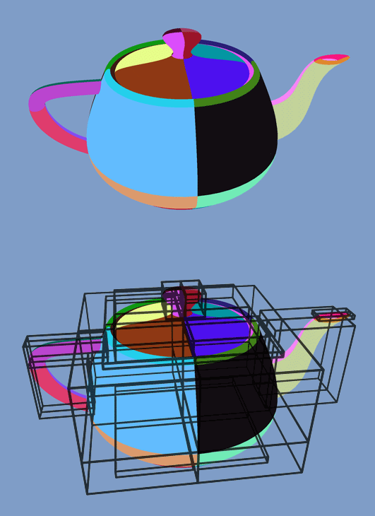
The simplest method to accelerate ray tracing can't necessarily be considered as an acceleration structure, however this is certainly the simplest way to cut down render times. Each one of the grid from the teapot has potentially more than a hundred triangles: with 8 divisions, the grid contains 128 triangles, which requires a similar number of intersection test for each ray cast into the scene. What we can do instead, is ray trace a box containing all the vertices of the grid. Such box is called a bounding volume:it is the tightest possible volume (a box in that case but it could also be a sphere) surrounding the grid. Figure 1 shows the bounding boxes of each one of the 32 Bézier patches making up the teapot model.


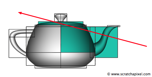
We can first test if the ray intersects this box, and if it doesn't, we know for sure that it can't intersect the geometry contained in this bounding volume (figure 2). If we can ignore the triangles from this bounding box, we save 128 ray-triangle intersection tests. Considering that many of the bounding boxes from the scene are likely to fail this test as well, overall, we can save a significant number of calls to the ray-triangle routine. If the ray intersects the bounding box though, all the triangles contained in the volume will have to be tested for an intersection with this ray. In figure 2, we can see a ray intersecting the bounding boxes of the Bézier patches making up the teapot model. Only colored boxes are intersected by the ray, and only the grids contained by these boxes will be tested for an intersection with the ray. Patches contained by the boxes which are not intersected can be safely rejected.
The following pseudocode illustrates this process:
for (each object in scene) {
    if (intersect(ray, object->boundingBox) == true) {
        for (each triangle in object) {
            if (intersect(ray, triangle) == true) {
                // the ray intersects the triangle
                ...
            }
        }
    }
}

Calculating a bounding box for an object is very simple. We can loop over all the vertices making up the mesh to find the minimum and maximum value for each of the point's coordinate (the xyz points position). These values form what we call the object's minimum and maximum extent and define the two corners of the bounding box (see figure 3). The bounding box of an object is usually computed when the object is built (for instance in the constructor of the polygon mesh class) and stored in a member variable of the object's class (each primitive type may require a different method to compute this bounding box. The bounding volume of a quadratic sphere for instance can be computed from its radius). The following code snippet from the ray tracer shows how we compute the bounding box of a polygon object (line 13). The bbox variable is a member variable of the base Object class (the code is available in the last chapter of this lesson).
class PolygonMesh : public Object
{
public:
    PolygonMesh(
        const Matrix44f &o2w,
        const uint32_t &np, const uint32_t *nv, const uint32_t *v,
        const Vec3f *pts, const Vec3f *nors = NULL) :
        Object(o2w), ntris(0), tris(NULL), P(NULL), N(NULL)
    {
        ...
        for (uint32_t i = 0; i < maxVertIndex + 1; ++i) {
            objectToWorld.multVecMatrix(pts[i], P[i]);
            bbox.extendBy(P[i]);
        }
        ...
    }
};

template<typename T, uint32_t D>
class Box
{
public:
    ...
    void extendBy(const Vec<T, D>& pt)
    {
        for (size_t i = 0; i < D; ++i) {
            if (pt[i] < bounds[0][i]) bounds[0][i] = pt[i];
            if (pt[i] > bounds[1][i]) bounds[1][i] = pt[i];
        }
    }
    ...
};
The rest of the code is very simple. We will use the ray-box intersection routine we have studied in lesson 7 (Intersecting Simple Shape):
uint64_t numRayBoxTests = 0;


template<typename T, uint32_t D>
bool Box<T, D>::intersect(const Ray<T>& r) const
{
    __sync_fetch_and_add(&numRayBoxTests, 1);
    ...
    return true;
}
We use the same as with the ray-triangle intersection method to count the number of times the ray-box intersection method has been called. A global variable numRayBoxTests declared in the box.cpp file is incremented using an atomic add operation each time the box intersect method is called. The final value is printed out at the end of the render with the other statistics.
We also created an AccelerationStructure base class which behaves very similarly to an objects. It holds an intersect method looping over all the objects from the scene (line 5). We first test for an intersection between the ray and the bounding box of the current object (line 7). If the test is successful, the ray is then tested against the object contained by the box (line 9). The rest of the code is very similar to the implementation of the trace function from lesson 11. Each time a triangle is intersected, we need to update the closest distance to the intersection point (lines 10-11) and keep a pointer to the intersected object (line 12):
const Object* AccelerationStructure::intersect(const Ray<float>& ray, IsectData& isectData) const
{
    float tClosest = ray.tmax;
    Object *hitObject = NULL;
    for (size_t i = 0; i < rc->objects.size(); ++i) {
        Ray<float> r(ray);
        if (rc->objects[i]->bbox.intersect(r)) {
            IsectData isectDataCurrent;
            if (rc->objects[i]->intersect(ray, isectDataCurrent)) {
                if (isectDataCurrent.t < tClosest && isectDataCurrent.t > ray.tmin) {
                    isectData = isectDataCurrent;
                    hitObject = rc->objects[i];
                    tClosest = isectDataCurrent.t;
                }
            }
        }
    }

    return (tClosest < ray.tmax) ? hitObject : NULL;
}
Finally we need to update the trace function. Rather than looping over all the objects from the scene, we just need to call the intersect method from the AccelerationStructure class. If this method returns a valid pointer to an object from the scene, an intersection occurred and we can set the color of the pixel with the intersected object's color:
template<typename T>
void trace(const Ray<T> ray, const RenderContext *rc, Spectrum &s)
{
    IsectData isectData;
    const Object *hitObject = NULL;
    if ((hitObject = rc->accelStruct->intersect(ray, isectData)) != NULL)
        s.xyz = hitObject->color;
    else
        s.xyz = rc->backgroundColor;
}
If we render the scene we used in the previous chapter, we now get the following statistics:
Render time                                 : 3.96 (sec)
Total number of triangles                   : 16384
Total number of primary rays                : 307200
Total number of ray-triangles tests         : 129335296
Total number of ray-triangles intersections : 111889
Total number of ray-box tests               : 9830400
Render time was reduced by a factor of about 34. Logically the ratio between the number of ray-triangle tests performed with and without this basic acceleration structure is about the same: 38. The two number are not exactly the same because of the extra time it now takes to compute the ray-box intersections (9.83 million times). However the benefits we get from using this scheme largely outweighs the additional work these tests require.
The technique presented in this chapter works well in the case of the teapot because the model contains many grids whose resolution (in terms of polygon count) is reasonably low. The ape model on the other hand, is very complex and is made of one single piece. If we were to render this object, we would only save time when the primary rays don't intersect its bounding box (which is, for a typical frame, maybe less than a third of the total number of pixels). For all the over rays, we would still have to perform an intersection test against the hundred thousand triangles making up the model. In that particular case, the bounding box method would only bring a small benefit compared to the brute force approach. It is simple and fast to implement but is clearly not adapted to all situations and for this reason it is not considered as a very good acceleration method.
The idea of using a bounding volume to accelerate ray tracing is quite old. It is hard to find exactly who and when the idea was proposed. In a paper from 1980 entitled "A 3-Dimensional Representation for Fast Rendering of Complex Scenes", the authors Ruben and Whitted already speak about the possibility of using a hierarchy of such bounding volumes for "fast" rendering (see references section at the end of this lesson).
What's Next?
In the next chapter we will present a technique presented by Kajiya and Kay in 1986 to accelerate ray tracing. This method is based on what's now known as bounding voume hierarchy (or BVH).