Bounding Volume Hierarchy: BVH (part 2)
Reading time: 20 mins.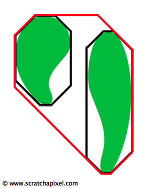
The rest of Kay and Kajiya's paper is focused on improving their technique by grouping the bounding volumes we have described in the previous chapter into a hierarchy of bounding volumes. This technique is called a Bounding Volume Hierarchy or BVH. It generally provides (compared to other possible acceleration structures) very good results. Many variations based on this principle exist. In this chapter we will look at the method used and described by Kay and Kajiya. The idea of grouping bounding volumes into larger volumes which we themselves group, etc. is very simple and also quite easy to understand. In figure 2, we are showing a group of objects associated with their respective bounding volumes (here a box for simplicity). By merging these bounding boxes together (usually by proximity) we obtain larger bounding volumes representing groups of objects. It is easy to see that if a ray doesn't intersect any of these larger groups, then we can avoid testing the volumes enclosed by these groups, possibly rejecting many objects at once. This obviously, saves a lot of render time.
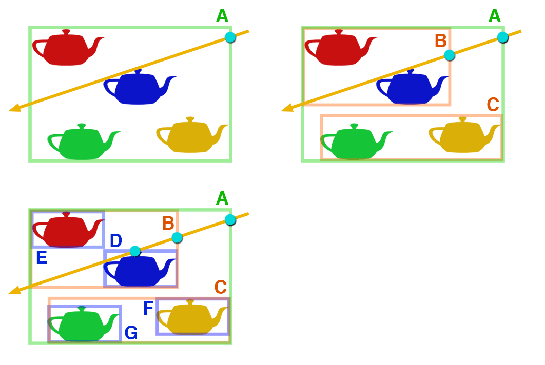
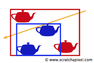
The principle is very simple however to be efficient, the objects and the volumes have to be grouped by proximity. The problem if they are not grouped by proximity, is illustrated in Figure 3. The two bounding boxes of the red teapots have been grouped together even though they are far away from each other. In Figure 3, the ray intersects the two bounding volumes and four teapots have to be tested for an intersection with the ray. In figure 1, only two of these teapot are tested for an intersection (D and E).
To group objects by proximity, Kay and Kajiya propose to insert them in a space partitioning data structure. This structure partitions space in sub-regions and objects are inserted in these sub-regions usually based on their position. The process is illustrated in Figure 3. If we create a box which encloses all the objects of the scene then we can subdivide this box in eight equally sized sub-boxes (in Figures 4 and 5, this process is illustrated in 2D). Each object of the scene can then be inserted (in the order they have been added to the scene) in the sub-boxes they overlap. We can then assume that all the objects contained in one of the sub-voxels are pretty close to each other (at least closer than the objects which are in the other sub-boxes).
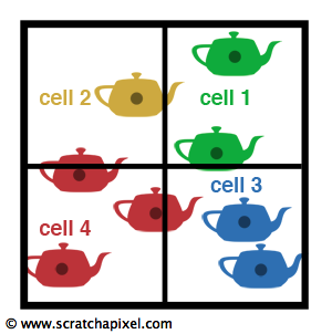
As you can see in figure 4, an object may overlap several sub-boxes or cells. In that case, Kay and Kajiya arbitrarily insert the object in one of the overlapped cells. We have chosen to insert them in the cell in which lies the object's bounding box centroid (represented by the dot in the center of each teapot). Two spatial data structures are proposed in the paper: a median cut and an octree. The first is related somehow to the k-d tree space partitioning data structure which you may have heard about. We won't be presenting these structures in this lesson. The latter, the octree, will be used in our implementation of Kay's and Kajiya's paper. As described before, it partitions a cube into eight cells which are themselves subdivided etc. The recursion process stops when all the objects have been inserted in the octree or when we reach a maximum user-defined depth.
Building the Hierarchy
The octree data structure is presented in detail in an other lesson. However, in short, the process for the creation and insertion of the object is the following. First we compute the bounding volumes of all the objects in the scene and as we go, we compute the overall scene bounding volume which is the result of these volumes combined. From that scene overall volume we can define the size of the octree (a cube located at the center of the overall volume, whose dimension is the maximum value of any of the volume's extent along the x- y- and z-axis). This cube represents the top node of the octree, its root. When we then insert objects in this octree, we traverse the tree in a top-down fashion. If the node in which we want to insert an object is a leaf, and that the leaf doesn't contain any object yet, then we insert the object in this node. If the node already contains an object (and unless we have reached a maximum user defined depth) then the current node is split in eight cells and the object contained by the node as well as the new object are inserted in the cells (note the object may overlap more than one cell) they overlap.
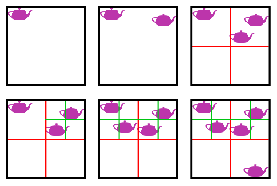
This process is repeated until all the objects are inserted in the octree. In a second step, the octree is traversed in a bottom-up fashion this time. We start from the leaves, and compute the overall bounding box of the objects they contain (a leaf can have one or more objects). The overall volume box of the node above the leaves is then computed from combining its children bounding volumes. This process is repeated until we reach the root (which at this point should be the same as the extent of the overall scene we have computed earlier on). At the end of these two processes, we obtain a representation of the scene as a hierarchy of bounding volumes, where the volumes are grouped based on proximity (objects contained in the leaves of a node are grouped together, etc.). Note that the ochre is actually not used as an acceleration structure (do not confuse this technique with the octree used as an acceleration structure - we will write a lesson on this technique in the future). The octree is actually of no real benefit for the ray-intersection tests. It is only used to compute and build this hierarchy of volumes. ## Intersecting the Hierarchy
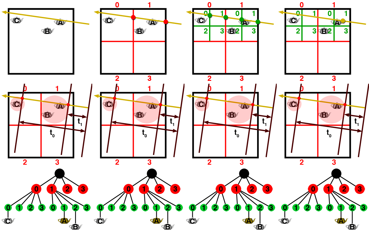
The intersection of the BVH is quite simple. We start from the root node and test if the ray intersects the bounding volume for this node. Generally, if the bounding volume of a node is intersected by the ray, we go one level down in the tree and test for an intersection with the bounding volumes of this node's children. If the node is a leaf, we test if the ray intersects any of the objects it contains. This solution is quite simple to implement however, it can be further optimized. When we test for the intersection of a ray with the bounding volumes of a node's children, assuming that the bounding volumes of more than one of these cells have been intersected, we should first investigate the children of the node with the smallest intersection distance, as the visible object is most likely to be contained in these cells. This idea is illustrated in figure 6 (we have represented the intersection with the bounding volume of a cell by a point at the intersection of the ray with the cell's boundaries. Keep in mind that in reality, we have an intersection with the bounding volume of the cell, represented by spheres in the figure, not the cell itself). As you can see, the ray intersects the root node (in black) which leads to testing the root's children (in red). The cells are tested in the order they have been created: 0, 1, 2, 3. The ray intersects the bounding volumes of cell 0 and 1 and therefore the children of these nodes are tested next. However the problem is that the children of the cells 0 will be tested before the children of cell 1 even though the intersection distance with the bounding volume from cell 1 (\(t_1\)) is smaller than the intersection distance with the volume from cell 0 (\(t_0\)). It would be more efficient to first test the children from cell 1 before testing the children from cell 0 as it would lead to finding the intersection with the teapot A sooner. Kay and Kajiya propose to use a list in which the node's children which are pierced by the ray are inserted and sorted according to their intersection distance (from the smallest to the largest). We then remove the first node from this list and test its children. If any of these children are intersected by the ray, they get themselves inserted to the list. They will be inserted in front of the existing elements from the list since their intersection distance is necessarily smaller than the intersection distance of any of the nodes already inserted.
In programming such lists are called priority queues. They are like regular queues where each element has a "priority" associated with it. In a priority queue, an element with high priority is served before an element with low priority. If two elements have the same priority, they are served according to their order in the queue. In our particular case, we will use the intersection distance to the bounding volume to define the priority of the volumes in the queue: the volume with the smallest intersection distance is the element from the queue with the highest priority. In C++ we can use the priority_queue class which is part of the STL C++ standard (see the source code section for more details).
By following this process, we are sure to always test the nodes from the hierarchy which are the closest to the ray's origin first. If these nodes do not contained the visible object, we then keep going by testing the nodes which are further away from the ray's origin, etc. until the list is empty.
while (priority_queue is not empty) {
    Node node = get node from the priority_queue with highest priority (and remove it)
    if node is a leaf
        for each object contained in node
            if object is intersected by ray
                 keep this object as potential visible object
        if an object was intersected
            return
    else
        // keep traversing the hierarchy by looking down the node's children
        for each children in node
            if node's children is intersected by ray at distance t
                insert node into priority_queue (use intersection distance t to define priority of the node in the list)
}
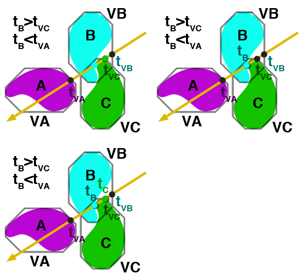
There is one last detail we need to be careful about. If you look at figure 7, you can see that we can't use the intersection distance to the bounding volumes to decide for certain which ones of these volumes contain the visible object. Even though the distance to the bounding volume of B \(t_{VB}\) is lower than the distance to the bounding volume of C \(t_{VC}\), the object that the ray will intersect is C and not B. We only know for certain that we can stop the traversal of the hierarchy when the distance to the intersected object, is lower than the intersection distance to the bounding volume of the next node in the list. As illustrated in figure 7, the nodes in the priority list should be in the following order VB, VC, VA (because \(t_{VB}\) < \(t_{VC}\) < \(t_{VA}\)). When we intersect the object contained by VB (the bounding volume for B) we find the intersection distance \(t_B\) for the object B. However \(t_B\) is not smaller than \(t_{VC}\) therefore we also have to test for the intersection with the object C and we find that \(t_C\) is lower than \(t_B\) therefore C becomes the potential intersected object instead of B. But because \(t_C\) is lower than \(t_{VA}\) we don't need to test for an intersection with A nor do we need to test for an intersection with any of the nodes which might be in the list after VA. We can therefore stop the hierarchal traversal and return B as the visible object. If we use all these techniques in our ray tracer we now get the following results:
Render time                                 : 1.61 (sec)
Total number of triangles                   : 16384
Total number of primary rays                : 307200
Total number of ray-triangles tests         : 41341952
Total number of ray-triangles intersections : 59017
Total number of ray-volume tests            : 1531064
The render is now 1.8 times faster (compared to the render from the previous chapter). The number of ray-volumes tests is reduced by 6.4 (proving that the bounding volume hierarchy is very efficient), the number of ray-triangle tests by 1.95 and the number of ray-triangle intersection by 1.89.
Source Code
The complete source code is available in the last chapter of this lesson.
The BVH class has become more complex. We have added to the class an OctreeNode and an Octree class. Readers interested in learning about octaves are referred to following sections where they can find a lesson on this topic. The octree node holds eight pointers to other octree nodes which are its children. The class constructors takes the scene extent as an input parameter (line 38). This extent is used to compute and set the root node's dimension and position (its centroid. Lines 40-49). New objects (more precisely their bounding volume, but remember that the Extents class holds a pointer to the enclosed object) are inserted from the root node (lines 52-53). If the current node is a empty leaf (no objects had been inserted in this leaf yet), we insert the object in this leaf and return. If the node is a leaf and contains at least one or more object(s) but that we have reached the octree maximum depth, we nevertheless insert the object in this node (line 73). However, if we haven't reached the maximum depth yet, we tag the node as "internal" and re-insert the object already held by the node as well as the new object in the octree (lines 77-82). If the node is not a leaf, we check in which children from the node the object should be inserted in (lines 86-93). If the child doesn't exist yet we create it (lines 97-98) and finally we insert the object into this child node (line 99). The function for building the hierarchy of volumes is simple. We start from the root and go down the tree until we reach the leaf nodes. The bounding volume of this node is computed by combining the bounding volumes of all the objects it keeps a pointer to. Then, as we move back up again, the bounding volume of the current node is computed by combining the bounding volumes of its children (line 130).
class BVH : public AccelerationStructure
{
    static const uint8_t kNumPlaneSetNormals = 7;
    static const Vec3f planeSetNormals[kNumPlaneSetNormals];
    struct Extents
    {
        Extents()
        {
            for (uint8_t i = 0; i < kNumPlaneSetNormals; ++i)
                d[i][0] = kInfinity, d[i][1] = -kInfinity;
        }
        void extendBy(const Extents &extents)
        {
            for (uint8_t i = 0; i < kNumPlaneSetNormals; ++i) {
                if (extents.d[i][0] < d[i][0]) d[i][0] = extents.d[i][0];
                if (extents.d[i][1] > d[i][1]) d[i][1] = extents.d[i][1];
            }
        }
        bool intersect(
            const float *precomputedNumerator, const float *precomputeDenominator,
            float &tNear, float &tFar, uint8_t &planeIndex);
        float d[kNumPlaneSetNormals][2]; // d values for each plane-set normals
        const Object *object; // pointer contained by the volume (used by octree)
    };
    Extents *extents;
    struct OctreeNode
    {
        OctreeNode *child[8];
        std::vector<const Extents *> data;
        Extents extents;
        bool isLeaf;
        uint8_t depth; // just for debugging
        OctreeNode() : isLeaf(true) { memset(child, 0x0, sizeof(OctreeNode *) * 8); }
        ~OctreeNode() { for (uint8_t i = 0; i < 8; ++i) if (child[i] != NULL) delete child[i]; }
    };
    struct Octree
    {
        Octree(const Extents &extents) : root(NULL)
        {
            float xdiff = extents.d[0][1] - extents.d[0][0];
            float ydiff = extents.d[1][1] - extents.d[1][0];
            float zdiff = extents.d[2][1] - extents.d[2][0];
            float dim = std::max(xdiff, std::max(ydiff, zdiff));
            Vec3f centroid(
                (extents.d[0][0] + extents.d[0][1]),
                (extents.d[1][0] + extents.d[1][1]),
                (extents.d[2][0] + extents.d[2][1]));
            bounds[0] = (Vec3f(centroid) - Vec3f(dim)) * 0.5f;
            bounds[1] = (Vec3f(centroid) + Vec3f(dim)) * 0.5f;
            root = new OctreeNode;
        }
        void insert(const Extents *extents)
        { insert(root, extents, bounds[0], bounds[1], 0); }
        void build()
        { build(root, bounds[0], bounds[1]); }
        ~Octree() { delete root; }
        struct QueueElement
        {
            const OctreeNode *node; // octree node held by this node in the tree
            float t; // used as key
            QueueElement(const OctreeNode *n, float thit) : node(n), t(thit) {}
            // comparator is > instead of < so priority_queue behaves like a min-heap
            friend bool operator < (const QueueElement &a, const QueueElement &b) { return a.t > b.t; }
        };
        Vec3f bounds[2];
        OctreeNode *root;
    private:
        void insert(
            OctreeNode *node, const Extents *extents,
            Vec3f boundMin, Vec3f boundMax, int depth)
        {
            if (node->isLeaf) {
                if (node->data.size() == 0 || depth == 16) {
                    node->data.push_back(extents);
                }
                else {
                    node->isLeaf = false;
                    while (node->data.size()) {
                        insert(node, node->data.back(), boundMin, boundMax, depth);
                        node->data.pop_back();
                    }
                    insert(node, extents, boundMin, boundMax, depth);
                }
            } else {
                // insert bounding volume in the right octree cell
                Vec3f extentsCentroid = (
                    Vec3f(extents->d[0][0], extents->d[1][0], extents->d[2][0]) +
                    Vec3f(extents->d[0][1], extents->d[1][1], extents->d[2][1])) * 0.5;
                Vec3f nodeCentroid = (boundMax + boundMin) * 0.5f;
                uint8_t childIndex = 0;
                if (extentsCentroid[0] > nodeCentroid[0]) childIndex += 4;
                if (extentsCentroid[1] > nodeCentroid[1]) childIndex += 2;
                if (extentsCentroid[2] > nodeCentroid[2]) childIndex += 1;
                Vec3f childBoundMin, childBoundMax;
                Vec3f boundCentroid = (boundMin + boundMax) * 0.5;
                computeChildBound(childIndex, boundCentroid, boundMin, boundMax, childBoundMin, childBoundMax);
                if (node->child[childIndex] == NULL)
                      node->child[childIndex] = new OctreeNode, node->child[childIndex]->depth = depth;
                insert(node->child[childIndex], extents, childBoundMin, childBoundMax, depth + 1);
            }
        }
        void computeChildBound(
            const uint8_t &i, const Vec3f &boundCentroid,
            const Vec3f &boundMin, const Vec3f &boundMax,
            Vec3f &pMin, Vec3f &pMax) const
        {
            pMin[0] = (i & 4) ? boundCentroid[0] : boundMin[0];
            pMax[0] = (i & 4) ? boundMax[0] : boundCentroid[0];
            pMin[1] = (i & 2) ? boundCentroid[1] : boundMin[1];
            pMax[1] = (i & 2) ? boundMax[1] : boundCentroid[1];
            pMin[2] = (i & 1) ? boundCentroid[2] : boundMin[2];
            pMax[2] = (i & 1) ? boundMax[2] : boundCentroid[2];
        }
        // bottom-up construction
        void build(OctreeNode *node, const Vec3f &boundMin, const Vec3f &boundMax)
        {
            if (node->isLeaf) {
                // compute leaf node bounding volume
                for (uint32_t i = 0; i < node->data.size(); ++i) {
                    node->extents.extendBy(*node->data[i]);
                }
            }
            else {
                for (uint8_t i = 0; i < 8; ++i)
                    if (node->child[i]) {
                        Vec3f childBoundMin, childBoundMax;
                        Vec3f boundCentroid = (boundMin + boundMax) * 0.5;
                        computeChildBound(i, boundCentroid, boundMin, boundMax, childBoundMin, childBoundMax);
                        build(node->child[i], childBoundMin, childBoundMax);
                        node->extents.extendBy(node->child[i]->extents);
                    }
                }
            }
        }
    };
    Octree *octree;
public:
    BVH(const RenderContext *rcx);
    const Object* intersect(const Ray<float> &ray, IsectData &isectData) const;
    ~BVH();
};
In the intersect method of the BVH class (line 37) we first test if the ray intersects the bounding volume of the entire scene (the extent of the ochre's root node). If it does we initialise a priority_queue list with this node and the intersection distance from the ray's origin to its bounding volume. We overloaded the operator < (line 63 above) to make it behave like a min heap (by default it behaves like a max heap setting the element with the highest key value with the highest priority. We want the opposite). The rest of the code is similar to the pseudocode given above. We take take the first node on top of the list (which we also remove from the list. Lines 72-73). If this node is a leaf then we test if the ray intersects any of the objects contained by the node and we keep track of the intersection minimum distance (line 79). If it is an internal node, we test if the ray intersect the bounding volumes of the node's children, and when it does, we add the child node to the list (using the intersection distance as the key to set the element's priority in the list. Line 93). This process is repeated until the list is empty but can be stopped sooner if the intersection distance of the list's first node is greater than the distance to the intersected object (line 71).
BVH::BVH(const RenderContext *rcx) : AccelerationStructure(rcx), extents(NULL), octree(NULL)
{
    Extents sceneExtents;
    extents = new Extents[rcx->objects.size()];
    for (uint32_t i = 0; i < rcx->objects.size(); ++i) {
        for (uint8_t j = 0; j < kNumPlaneSetNormals; ++j) {
            rcx->objects[i]->computeBounds(planeSetNormals[j], extents[i].d[j][0], extents[i].d[j][1]);
        }
        extents[i].object = rcx->objects[i];
        sceneExtents.extendBy(extents[i]);
    }
    // create hierarchy
    octree = new Octree(sceneExtents);
    for (uint32_t i = 0; i < rcx->objects.size(); ++i) {
        octree->insert(extents + i);
    }
    octree->build();
}

inline bool BVH::Extents::intersect(
    const float *precomputedNumerator, const float *precomputeDenominator,
    float &tNear, float &tFar, uint8_t &planeIndex)
{
    __sync_fetch_and_add(&numRayVolumeTests, 1);
    for (uint8_t i = 0; i < kNumPlaneSetNormals; ++i) {
        float tn = (d[i][0] - precomputedNumerator[i]) / precomputeDenominator[i];
        float tf = (d[i][1] - precomputedNumerator[i]) / precomputeDenominator[i];
        if (precomputeDenominator[i] < 0) std::swap(tn, tf);
        if (tn > tNear) tNear = tn, planeIndex = i;
        if (tf < tFar) tFar = tf;
        if (tNear > tFar) return false;  //test for an early stop
    }

    return true;
}

const Object* BVH::intersect(const Ray<float> &ray, IsectData &isectData) const
{
    const Object *hitObject = NULL;
    float precomputedNumerator[BVH::kNumPlaneSetNormals], precomputeDenominator[BVH::kNumPlaneSetNormals];
    for (uint8_t i = 0; i < kNumPlaneSetNormals; ++i) {
        precomputedNumerator[i] = dot(planeSetNormals[i], ray.orig);
        precomputeDenominator[i] = dot(planeSetNormals[i], ray.dir);;
    }
#if 0
    float tClosest = ray.tmax;
    for (uint32_t i = 0; i < rc->objects.size(); ++i) {
        __sync_fetch_and_add(&numRayVolumeTests, 1);
        float tNear = -kInfinity, tFar = kInfinity;
        uint8_t planeIndex;
        if (extents[i].intersect(precomputedNumerator, precomputeDenominator, tNear, tFar, planeIndex)) {
            IsectData isectDataCurrent;
            if (rc->objects[i]->intersect(ray, isectDataCurrent)) {
                if (isectDataCurrent.t < tClosest && isectDataCurrent.t > ray.tmin) {
                    isectData = isectDataCurrent;
                    hitObject = rc->objects[i];
                    tClosest = isectDataCurrent.t;
                }
            }
        }
    }
#else
    uint8_t planeIndex = 0;
    float tNear = 0, tFar = ray.tmax;
    if (!octree->root->extents.intersect(precomputedNumerator, precomputeDenominator, tNear, tFar, planeIndex)
        || tFar < 0 || tNear > ray.tmax)
        return NULL;
    float tMin = tFar;
    std::priority_queue<BVH::Octree::QueueElement> queue;
    queue.push(BVH::Octree::QueueElement(octree->root, 0));
    while(!queue.empty() && queue.top().t < tMin) {
        const OctreeNode *node = queue.top().node;
        queue.pop();
        if (node->isLeaf) {
            for (uint32_t i = 0; i < node->data.size(); ++i) {
                IsectData isectDataCurrent;
                if (node->data[i]->object->intersect(ray, isectDataCurrent)) {
                    if (isectDataCurrent.t < tMin) {
                        tMin = isectDataCurrent.t;
                        hitObject = node->data[i]->object;
                        isectData = isectDataCurrent;
                    }
                }
            }
        }
        else {
            for (uint8_t i = 0; i < 8; ++i) {
                if (node->child[i] != NULL) {
                    float tNearChild = 0, tFarChild = tFar;
                    if (node->child[i]->extents.intersect(precomputedNumerator, precomputeDenominator,
                        tNearChild, tFarChild, planeIndex)) {
                        float t = (tNearChild < 0 && tFarChild >= 0) ? tFarChild : tNearChild;
                        queue.push(BVH::Octree::QueueElement(node->child[i], t));
                    }
                }
            }
        }
    }
#endif

    return hitObject;
}
Normally, the objects which we should insert in the BVH are the triangles not the meshes. In order to complete the basic section as quickly as possible, we will explain how this can be done in a future version of this lesson. In the next chapter though, we will show how to insert the triangles in a grid acceleration structure. As an exercise, you can try to modify the code of the BVH found in this lesson to support the insertion of triangles, by taking example on the grid implementation.
What's Next?
Kay and Kajiya's technique gives excellent results with the teapot scene. Generally BVH method perform well and are used sometimes in production renderers as the choice of supported accelerated structure (usually in combination with another structure for a reason that will become clear at the end of the next chapter). The idea is to break these models somehow into smaller pieces which are inserted in the voxels a simple 3D grid. As we will show in the next chapter, ray tracing grids is simple and fast.