Basic Implementation
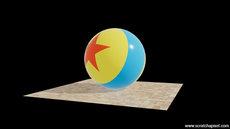
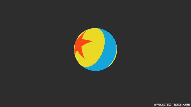
Reading time: 35 mins.As a sneak peek, here is the image that our program will output, where both the ball and the plane in this example have their colors textured. In this chapter, we will learn how this can be done in practice with a simple implementation of texture mapping applied to the shader color parameter.
How does this work
The principle is surprisingly simple. The idea behind texture mapping is based on associating each vertex of a polygonal mesh with a 2D coordinate that indicates a position within the texture. These coordinates are defined as floats, though, of course, the coordinates of an image are defined in terms of pixels. Texture coordinates are generally (though not always, as we will see at the end of the lesson) within the range [0,1]. When this is the case, we say that the texture coordinates are normalized. We will see at the end of the lesson that it is not necessary for these textures to be normalized, and in fact, this is no longer the norm for production assets (the complex models used in special effects films or animated films such as those by Pixar or Disney). We will explain why.
Let's take the example of a quad to start with something simple. Typically, the texture coordinate (0,0) corresponds to the bottom-left corner of the image, while the texture coordinate (1,1) corresponds to the top-right corner. If we imagine a quad with four vertices having coordinates v0={-1,0,-1}, v1={-1,0,1}, v2={1,0,1}, and v3={1,0,-1}, we can assign each of these vertices the texture coordinates uv0={0,0}, uv1={1,0}, uv2={1,1}, and uv3={0,1}.
Note that texture coordinates are most often denoted by the letters uv or st. It’s common to refer to "uvs" or "st coordinates" instead of "texture coordinates." While the exact origin of these terms isn't certain, it's a common practice in mathematics to use s and t or u and v as coordinates over parametric surfaces, such as NURBS or Bézier patches. Since texture coordinates are also 2D coordinates that define a position on a surface (but in texture space rather than geometric space), it's no surprise that early computer graphics researchers adopted these letters to refer to texture coordinates as well.
Note that most graphics APIs use the term st rather than uv. However, interestingly, most software refers to a UV editor, and artists tend to talk about UV unwrapping rather than ST unwrapping, so the terminology is a bit inconsistent. But, just to be clear, these two terms mean exactly the same thing—they are interchangeable.
When I say that texture coordinates refer to a position on the surface in texture space, I should clarify what this means. We started with a simple example using a quad, but how does this work with a cube, a sphere, or any other arbitrary shape? This is where texturing becomes more complex. You need to "unfold" or "unwrap" the 3D object to make it flat so that you can map your texture onto it. For a cube, there's a relatively straightforward solution since a cube can be unfolded, as shown in the animation below. For other surfaces, like a sphere, it's more complicated. Unfolding a sphere to make it flat is a challenge almost as old as cartography, where the goal is to represent land and oceans distributed over the Earth's surface onto a flat map. We won't delve into the various solutions to this, but it's fairly easy to assign texture coordinates procedurally if necessary, though this doesn't always produce the best possible UVs. These are likely to cause the texture to pinch at the poles of the sphere. Avoiding texture pinching or any kind of distortion is really the main challenge in texture mapping.
To summarize, when rendering a textured object, note that we first apply one form of mapping where each vertex of the mesh is assigned a position on the flat 2D space of the image/texture. This is what we refer to as texture space. In technical papers, this step is also called parametrization. Then, we project the 3D object into the 2D screen space. These steps are important to mention because the underlying mapping process undergoes a few transformation steps:
-
The parametrization step: This step involves mapping the texture onto the surface of a 3D object. It describes the 3D vertices in terms of two parameters, \(u\) and \(v\) (or \(s\) and \(t\)). In fact, you may often see this expressed in various papers and resources as \((u,v) = T(x,y)\), where \((u,v)\) are the parameters resulting from a function \(T\) that takes the sample location coordinates \((x,y)\) as input.
-
The rendering process: This involves projecting that 3D object onto the 2D surface of a screen, during which the mapped texture undergoes a resampling process. This will become most obvious when we discuss filtering in the next chapter.
NURBS or Bézier surfaces, and more generally parametric surfaces, are excellent for texturing because, due to their parametric nature, texture coordinates can be generated on the fly during the process of converting the surface from its parametric form into polygons. The polygonalization of a parametric surface involves calculating surface positions at regular intervals along the s and t parametric coordinates. Once a 3D point is generated for these st or uv coordinates, we simply assign those coordinates to the vertex itself, which naturally becomes the surface's texture coordinates. As a result, there's no need for these surfaces to generate texture coordinates using a specialized UV editor, like those provided by 3D software (Maya, Blender, etc.), unlike polygonal meshes where it is necessary to create texture coordinates after the mesh is created.
Most polygonal meshes, however, have shapes that are not as simple as a cube or a sphere. So, what do we do then? Unfortunately, there is no simple solution to this problem. Generally, each 3D modeling tool, such as Blender or Maya, offers a UV editor with various methods to flatten the surface of a 3D object as effectively as possible. The problem of flattening a 3D model onto a 2D surface is a significant research topic because it is quite complex.
-
Technically, this process needs to preserve, if possible, the relative area of the polygons as well as their aspect ratio. Take the example of a rectangle: if the texture coordinates do not correspond to a rectangle with the same aspect ratio, then when the texture is applied, if the image used as a texture is not scaled accordingly, it will appear stretched when rendered (as shown in the following images).
-
Secondly, it’s crucial to avoid overlapping polygons.
-
Thirdly, it's preferable to keep the polygons attached to one another, as this simplifies the texture editing process. However, this isn't always possible. Think of the process like flattening out a sheepskin or cowhide to make a rug (thankfully, lion skins are a thing of the past). As you can see, cuts had to be made at the legs and the belly to make this flattening possible. The same principle applies to meshes, but deciding where to make these cuts to flatten the mesh "skin" in the most optimal way is not always straightforward.
-
Finally, it’s important to optimize the available texture space—specifically, the [0,0] to [1,1] area—so that the maximum number of texture pixels is used during the mapping process, ensuring optimal resolution in the final result.
Achieving a satisfactory result that meets all these constraints for meshes of arbitrary shapes is not simple. This process requires specialized artists, often the modelers themselves who created the mesh, and this work is called UV unwrapping or unfolding. This work is generally done in modeling software like Maya or Blender, using a tool called the UV editor. This editor typically offers several tools to flatten a mesh as effectively as possible, with relatively simple techniques like planar, cylindrical, cubic, or spherical mapping, as well as more sophisticated methods suited to complex meshes, such as the example of the sheep, the cow, a dinosaur from Jurassic Park, Woody from Toy Story, a Minion character, or King Kong—the problem would be the same. This is also a problem for modelers because any subsequent changes to the mesh require the UVs to be remade or at least adjusted. This wouldn’t be as much of an issue if it didn’t affect the existing painted textures, which themselves may need to be significantly repainted due to UV changes. These adjustments can trigger a domino effect, leading to additional manual work, which is why they incur a cost both in terms of time and money when these changes need to be made during production.
As a side note, it's interesting to note that the process of parametrization, which we mentioned earlier, is a type of affine transformation. This transformation converts the vertices of a planar polygon (e.g., a triangle or a parallelogram) in 3D space to coordinates in texture space, which is a 2D space. This can be effectively represented by the following equation:
$$ \begin{pmatrix} u \\ v \\ 1 \end{pmatrix} = M_{t0} \cdot \begin{pmatrix} x_o \\ y_o \\ z_o \\ 1 \end{pmatrix} $$This equation essentially states that the equivalent \(uv\) coordinates of a point in 3D space, defined by coordinates \(x, y, z\), can be obtained by multiplying the 3D point by the matrix \(M_{t0}\). If the positions of the 3D vertices forming a triangle in the UV plane are known, the coefficients of that matrix can be determined by solving a system of linear equations:
$$ M_{t0} = \begin{pmatrix} a & b & c & d \\ e & f & g & h \\ i & j & k & l \end{pmatrix} $$Each triangle or quadrilateral making up the mesh can have its own unique mapping. This is because the texture mapping on the surface can vary between different parts of the mesh. For instance, different triangles might map to different areas of the texture, or they might map to the same area but with different orientations or scales. Therefore, each triangle (or quad) will generally have its own unique 3x4 matrix \(M_{t0}\).
Now, this lesson is not focused on the science behind the parametrization step that leads to the generation of texture coordinates. However, it is important to be aware that parametrization is a topic in itself and can be quite mathematically involved (we should probably devote a lesson to this in the future). For this lesson, we assume that the UVs have already been generated using software like Maya or Blender and that the model we will be working with includes this topological information, such as the vertices that compose it, the list of indices that define the faces of the mesh, and its texture coordinates. With this being said, let’s take a closer look at how this information is presented.
A Practical Implementation: Basics
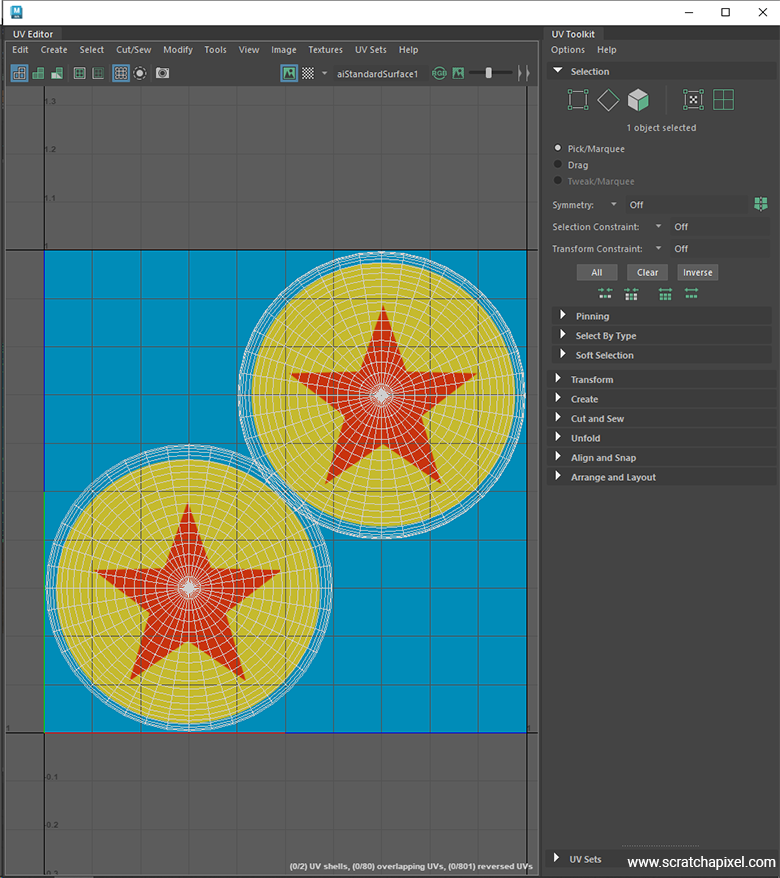
For our first example, we are going to render a sphere with some orientation, whose UV mapping has been done in Maya, a common digital content creation tool used by many professionals. The goal of this exercise is to recreate the textured ball from the Pixar Luxo short film, as mentioned in the previous chapter. The following image shows what the UVs look like in Maya's UV editor. We've applied planar mapping to each half of the sphere, allowing each hemisphere to receive a different pattern, though in our example, they will be identical. Note how some of the UVs overlap towards the center of the image. However, this isn't an issue because the vertices in question overlap a section of the texture filled with a uniform color.
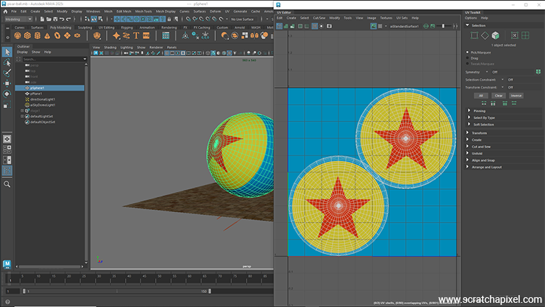
If you are not familiar with the concept of texture, this example will hopefully help you better understand it. As you can clearly see in this image, the vertices of the 3D sphere have been flattened. Another way, perhaps more accurate and less confusing, to describe it is to talk about a mesh whose vertices are in 2D instead of 3D. Each vertex of this 2D mesh corresponds to a vertex of the 3D mesh.
Now that we have a model with texture coordinates (and a texture), we will export the necessary data to render this model with our program.
Before we break down the process step by step, let's first provide an overview. If you look back at older computer graphics papers, you might find that they suggest different possible methods for achieving this. However, as they also point out, the method that was already most popular back then—and is almost universally adopted today—is referred to as the screen order method. This is the method used in this lesson.
The idea is that each pixel in screen space is inverse-transformed into texture space, and a pixel in the texture is read from that location. The process of transforming a pixel sample location (the pixel center for example if you use 1 sample per pixel) to \(st\) coordinates was described in the lesson on rasterization, notably in the chapter on Perspective Correct Interpolation and Vertex Attributes, so it won't be revisited here. However, it will be re-implemented in our sample code. What we will learn in this lesson focuses more on the process of reading the texture pixel values.
Step 1: Defining The Necessary Data
As you know, defining a polygonal mesh requires, at a minimum, a vertex array. This is followed by the face array count, which corresponds to the number of vertices that make up each face of the mesh. Finally, there's the index array, which provides the indices of each vertex for each face that composes the polygonal mesh.
For texture coordinate support, we will also need a texture coordinate array, but this time, these will be 2D points, not 3D points. Each texture coordinate corresponds to a position in image space, but in normalized coordinates, meaning they range from 0 to 1. There will be one texture coordinate per vertex in the mesh. While one might assume that the mapping (i.e., the correspondence between each of these texture coordinates and the vertices that make up the mesh) is the same as the index array of the faces, this is generally not the case. Therefore, it's important to understand that each texture coordinate array comes with its own index array, which maps each of the texture coordinates to the respective vertices of the mesh.
To summarize, for texture mapping support, we have two additional arrays on top of the three existing ones: the list of texture coordinates and the list of indices that will allow us to map each of these texture coordinates to a specific point on the mesh.
int faceVertexCounts[] = {4, 4, ... 3};

int faceVertexIndices[] = {0, 1, 41, 40, 1, 2, 42, 41, ... 1559, 1520, 1561};

point3f points[] = {{0.8900543, 0.7908807, 0.4050587}, {0.8934053, 0.7852825, 0.39461803}, ... {-0.8607362, 1.2789372, -0.42582545}};

texcoord2f st[] = {{0.3236586, 0.2969423}, {0.3228032, 0.29337937}, ... {0.6763413, 0.70305765}};

int indices[] = {0, 1, 2, 3, 1, 4, 5, 2, ... 762, 1580, 761};
In the example above, we have the following elements:
-
faceVertexCounts: This is an array where each element indicates how many vertices the face at that element index is composed of. -
faceVertexIndices: If the first face is composed of four vertices, the first four numbers of this array indicate the indices of these vertices in thepointsarray. -
points: This is the array of vertices, representing 3D positions. -
st: These are the texture coordinates, represented as 2D points. -
indices: Similar to thefaceVertexIndices, the first four numbers of this array represent the indices of the 4 vertices that make up the first face, in thestarray. As mentioned above, this allows us to define the texture coordinates in an order that is independent of the way they are stored in thepointsarray.
We will load this data into our mesh object. Remember, we first need to convert each face into triangles, a process we have already explained, so we won't revisit that. First, we calculate the total number of triangles we will end up with based on the faceVertexCounts. From there, we copy the points and st coordinates into their respective arrays and build a list of indices that will store the indices of the vertices making up each triangle in the mesh. Each group of three consecutive elements in these arrays represents the indices of a triangle: the indices of the triangles in the points array for the mesh->face_vertex_indices array, and the indices in the st array for the mesh->st.indices array. Here is the code that processes the mesh:
Note that for this lesson, we've decided to write the code in C (as much as possible). This was done as an exercise because we found it interesting to experience what it's like to write a C-compatible program as opposed to C++. Many of our friends have expressed frustration with C++ and have moved back to C, so we wanted to see for ourselves how it feels to write something in C (which is the langage I have been mostly using until the early 2000s) compared to C++. Additionally, within the context of Scratchapixel—a platform dedicated to education—it's not a bad idea to showcase code in a slightly different language. It helps you learn more ways of doing things.
Overall, since we are experienced with both C and C++, we encountered no surprises in making the switch. C is perfectly fine, but it requires you to manage most of the memory yourself, which increases the risk of memory leaks and crashes due to memory corruption. The benefit, however, is that you don’t rely on libraries that handle this for you, which can increase binary size and add other overhead. We won’t dive deeper into this debate—let’s just get on with it. C is just as good a language as C++. In fact, C is like the raw version of C++, much like AC/DC is to Britney Spears, or for the Gen Z crowd, Iron Maiden to Taylor Swift.
struct mesh {
	struct point3f* points;
	int* face_vertex_indices;
	struct {
		struct texcoord2f* coords;
		int* indices;
	} st;
	int num_triangles;
	int num_points;
	struct normal3f* normals;

	struct shader* shader;
};

static void create_mesh(struct context* const context, struct mesh* const mesh) {
#include "sphere.h"
	int num_faces = sizeof(faceVertexCounts) / sizeof(faceVertexCounts[0]);
	mesh->num_points = sizeof(points) / sizeof(points[0]);
	fprintf(stderr, "num points %d\n", mesh->num_points);
	mesh->points = (struct point3f*)malloc(sizeof(points));
	struct point3f* pts = mesh->points;
	memcpy((char*)pts, points, mesh->num_points * sizeof(struct point3f));

	for (int i = 0; i < mesh->num_points; ++i, ++pts) {
		point_mat_mult(pts, context->world_to_cam, pts);
	}

	mesh->num_triangles = 0;
	for (int i = 0; i < num_faces; ++i) {
		mesh->num_triangles += faceVertexCounts[i] - 2;
	}
	assert(mesh->num_triangles);

	mesh->face_vertex_indices = (int*)malloc(mesh->num_triangles * 3 * sizeof(int));
	mesh->st.indices = (int*)malloc(mesh->num_triangles * 3 * sizeof(int));

	int vert_index_array_size = sizeof(faceVertexIndices) / sizeof(faceVertexIndices[0]);
	int tex_index_array_size = sizeof(indices) / sizeof(indices[0]);
	int tex_coord_array_size = sizeof(st) / sizeof(st[0]);

	mesh->st.coords = (struct texcoord2f*)malloc(sizeof(st));
	memcpy((char*)mesh->st.coords, st, tex_coord_array_size * sizeof(struct texcoord2f));

	int vi[3], ti[3], index_offset = 0;
	int* pvi = mesh->face_vertex_indices;
	int* pti = mesh->st.indices;
	for (int i = 0; i < num_faces; ++i) {
		vi[0] = faceVertexIndices[index_offset]; ti[0] = indices[index_offset++];
		vi[1] = faceVertexIndices[index_offset]; ti[1] = indices[index_offset++];
		for (int j = 0; j < faceVertexCounts[i] - 2; ++j) {
			vi[2] = faceVertexIndices[index_offset]; ti[2] = indices[index_offset++];
			memcpy((char*)pvi, vi, sizeof(int) * 3);
			memcpy((char*)pti, ti, sizeof(int) * 3);
			vi[1] = vi[2];
			ti[1] = ti[2];
			pvi += 3; pti += 3;
		}

	}
	...
}
We now have a mesh with all the necessary data, not only for rendering the mesh itself—such as information about its vertices and how they connect to form triangles—but also for the mesh's texture coordinates. With this in place, we are ready to render the mesh.
Step 2: Rendering the Scene
The rest of the rendering process is quite straightforward because, regardless of the algorithm used—whether it's ray tracing or rasterization—the principle remains the same. For example, in ray tracing, we calculate the visibility of triangles by casting rays from the camera to check if these rays intersect the triangles that make up the mesh. We will then see how we can use the texture coordinates to determine the color of the pixel corresponding to the intersection point between the ray and the triangle.
First, let’s remember that each vertex of these triangles has texture coordinates assigned to it. The idea is quite simple: when we calculate the intersection of a ray and a triangle, as discussed in previous lessons on ray-triangle intersections, we return not only the distance between the ray's origin and the intersection itself (represented by the variable \(t\)), but also the barycentric coordinates of the intersection on the triangle. These barycentric coordinates allow us to interpolate any variable—also known as primitive variables—that is attached or assigned to the vertices of the triangle. In this case, we use them to interpolate the texture coordinates, determining the exact texture coordinates at the point where the ray intersects the triangle.
For this lesson, in addition to writing the code in C (as opposed to C++, which we typically use), we’ve also decided to employ the rasterization algorithm instead of ray tracing. Just as it’s beneficial to navigate between C and C++, it’s also valuable to explore both rasterization and ray tracing. While history (at least for now) shows that most rendering systems (including GPU architectures) are adopting ray tracing, 1) rasterization is still very common in games, 2) it produces images much faster than ray tracing (at least when solving the visibility problem in simpler scenes without complex shading), and 3) it involves techniques that are important to understand, such as the concepts of perspective divide and projection.
However, using rasterization introduces additional complexity when dealing with the interpolation of primitive variables and barycentric coordinates compared to ray tracing. In ray tracing, the process is straightforward: the barycentric coordinates obtained from the ray-triangle intersection can be directly used to interpolate any vertex or primitive variables because the intersection occurs in 3D object/world space. With rasterization, the process is more involved:
-
First, divide the texture (st) coordinates by their respective 3D vertex z-coordinates.
-
Then, calculate the barycentric coordinates for the screen-projected triangle.
-
Next, compute the interpolated depth for the current pixel samples using these barycentric coordinates and the triangle vertices' z-coordinates.
-
Afterward, interpolate the texture (st) coordinates using the barycentric coordinates.
-
Finally, project the interpolated texture (st) coordinates by multiplying them back by the interpolated depth value to correct for perspective projection distortion.
This process is explained in detail in the lesson on rasterization, particularly in the chapter on Perspective Correct Interpolation and Vertex Attributes. Please refer to that lesson if you need a refresher or an introduction to this algorithm. As a quick reminder, this approach is necessary to correct for perspective projection, which preserves lines but not distances. This technique is called vertex attribute perspective-correct interpolation, also known as rational-linear or hyperbolic interpolation. It's crucial to understand this process to achieve correct texture coordinates when working with a rasterizer.
What’s important here is that we obtain the texture (st) coordinates as a result of interpolating the texture coordinates attached to the triangle's vertices at the point on the triangle in 3D space, which, once projected onto the screen, is located at the center of the pixel. Our sample program uses a simple form of MSAA short for multi-sample anti-aliasing. We use 4 pixel samples, so in our case, this will be the location of samples offset from the pixel coordinates by {0.25, 0.25}, {0.75, 0.25}, {0.75, 0.25}, and {0.75, 0.75}, respectively.
Technically, if you refer to the Vulkan specification, for instance, you will see that the samples are typically slightly rotated. For a 2x2 pattern, the sample positions in the Vulkan specs are defined as (0.375, 0.125), (0.875, 0.375), (0.125, 0.625), (0.625, 0.875). Just as a note. Sampling is covered in a separate lesson.
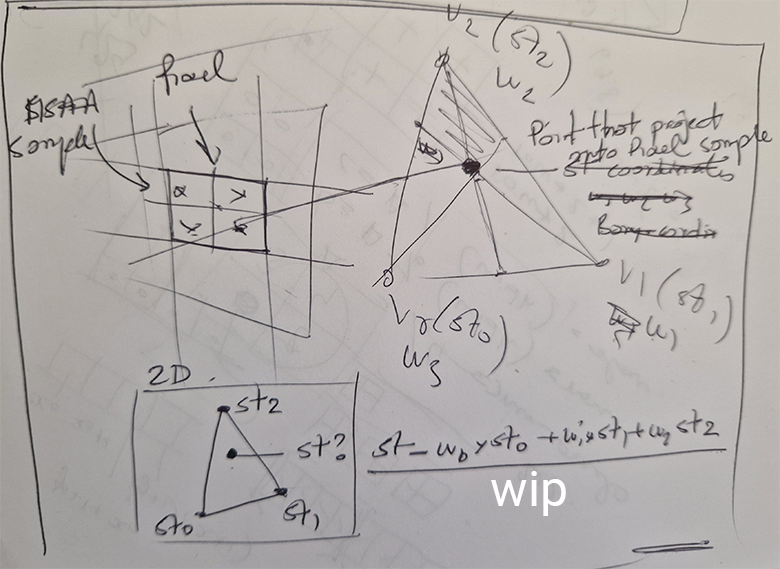
Whether you use ray tracing or rasterization, the goal remains the same: finding the point on the triangle's surface that corresponds to the center of each pixel in the image, or each pixel sample (if using MSAA). In ray tracing, you cast a ray through the center of the pixel to find the intersection point with the triangle. In rasterization, you project the triangle onto the screen and check if the pixel center (or pixel sample) lies within the triangle's edges. If it does, you interpolate the triangle's vertex positions to determine the corresponding 3D point on the triangle's surface. This step requires projecting the point back from screen space to camera space. Again this process is explained in detail in the lesson on rasterization. And we use the same method for interpolating any primitive variables. For this lesson, we are interested in finding what are the texture coordinates at this point on the triangle (Figure 1).
Here is the section of the code from our sample program responsible for calculating the triangle's st coordinates:
static inline void rasterize(int x0, int y0, int x1, int y1,
							 const struct point3f* const p0, const struct point3f* const p1, const struct point3f* const p2,
							 const struct texcoord2f* const st0, const struct texcoord2f* const st1, const struct texcoord2f* const st2,
							 const struct mesh* const mesh,
							 struct context* context) {
	float area = edge(p0, p1, p2);
	struct point3f pixel, sample;
	pixel.y = y0;
	for (int j = y0, row = y0 * context->extent.width; j <= y1; ++j, pixel.y += 1, row += context->extent.width) {
		pixel.x = x0;
		for (int i = x0, index = row + x0; i <= x1; ++i, pixel.x += 1, ++index) {
			for (int k = 0; k < num_samples; ++k) {
				sample.x = pixel.x + sample_pattern[k].x;
				sample.y = pixel.y + sample_pattern[k].y;

				float w0 = edge(p1, p2, &sample);
				float w1 = edge(p2, p0, &sample);
				float w2 = edge(p0, p1, &sample);

				if (w0 >= 0 && w1 >= 0 && w2 >= 0) {
					w0 /= area, w1 /= area, w2 /= area;
					float one_over_z = w0 / p0->z + w1 / p1->z + w2 / p2->z;
					float z = 1 / one_over_z;

					if (z < context->depth_buffer[index * num_samples + k]) {
						context->depth_buffer[index * num_samples + k] = z;

						struct texcoord2f st;
						st.s = st0->s * w0 + st1->s * w1 + st2->s * w2;
						st.t = st0->t * w0 + st1->t * w1 + st2->t * w2;
						st.s *= z;
						st.t *= z;
						shade(mesh->shader, st, &context->color_buffer[index * num_samples + k]);
					}
				}
			}
		}
	}
}
The astute reader will notice the call to the shade function, where we use the interpolated st coordinates to determine the color from the texture at these specific coordinates.
Step 3: Texture Lookup
Next, before we can look up the color of the texture at these specific texture coordinates, we first need a texture. This process will remain basic in our sample program. We will simply load the content of an image stored in the PPM file format, which you can find described in the lesson Digital Images: from File to Screen. You can open and save these images with programs like Photoshop or GIMP (which is free, though less user-friendly).
The structure of our program is fairly standard. Each mesh contains a pointer to a shader object that holds information regarding the surface appearance. Our basic shader will only hold (in the form of a union) a constant color and/or a pointer to an image, in case we decide to use a texture instead of the constant color. Below are the code snippets responsible for these tasks. Let's first look at the shader definition and implementation:
struct image {
    int width;
    int height;
    unsigned char* data;
};

struct shader {
    union color {
        struct color3f constant_value;
        struct image* image_ptr;
    } color;
};

struct mesh {
    struct point3f* points;
    int* face_vertex_indices;
    struct {
        struct texcoord2f* coords;
        int* indices;
    } st;
    int num_triangles;
    int num_points;
    struct normal3f* normals;
    struct shader* shader;
};
Here is the code snippet for allocating the shader and loading the texture:
void set_texture(struct image* const image, const char* filename) {
    FILE* file = fopen(filename, "rb");
    char format[3];
    int bpp;
    fscanf(file, "%2s", format);  // Content should be P6
    fscanf(file, "%d %d", &image->width, &image->height);
    fscanf(file, "%d", &bpp);
    fgetc(file);
    image->data = (unsigned char*)malloc(image->width * image->height * 3);
    fread(image->data, 3, image->width * image->height, file);
    fclose(file);
}

static void create_mesh(struct context* const context, struct mesh* const mesh) {
    #include "sphere.h"
    ...
    mesh->shader = (struct shader*)malloc(sizeof(struct shader));
    mesh->shader->color.image_ptr = (struct image*)malloc(sizeof(struct image));
    mesh->shader->color.image_ptr->data = NULL;
    set_texture(mesh->shader->color.image_ptr, "./pixar-texture3.pbm");
}
Good, so we have our st coordinates at the point on the triangle visible through the pixel, and we have a texture. The next step is to perform what we usually refer to as a texture lookup—a term that simply means "find the color of the texture at texture coordinates \(st\)." It’s not a particularly complex operation, but let's use the professional terminology. Let's perform a texture lookup!
Remember that texture coordinates are normalized, meaning they range from 0 to 1 (usually, though we will later see that this doesn't always have to be the case and discuss how to handle such scenarios). So, the first thing we need to do is convert these normalized texture coordinates into actual texture coordinates within the image. This conversion involves mapping the 0-1 range to pixel values.
This is a straightforward process. Since we know the dimensions of the texture, all we need to do is multiply the texture coordinates (the x and y values) by the texture's dimensions (width and height in pixels). This converts the normalized coordinates into pixel coordinates within the texture image, making sure to clamp the index values to the image's width and height minus one.
static void shade(const struct shader* shader, struct texcoord2f st, struct color3f* ci) {
	if (shader->color.image_ptr != NULL) {
		const struct image* const image = shader->color.image_ptr;
		struct point2i texel;
		texel.x = (int)fminf(st.s * image->width, image->width - 1);
		texel.y = (int)fminf((1 - st.t) * image->height, image->height - 1);
		unsigned char texel_color[3];
		memcpy(texel_color, image->data + (texel.y * image->width + texel.x) * 3, 3);
		ci->x = texel_color[0] / 255.f;
		ci->y = texel_color[1] / 255.f;
		ci->z = texel_color[2] / 255.f;
		return;
	}
	ci->x = shader->color.constant_value.x;
	ci->y = shader->color.constant_value.y;
	ci->z = shader->color.constant_value.z;
}
There's one detail to note regarding the code: we need to invert the st.t coordinates. If you look at how the coordinates are defined in the UV editor, you'll notice that the origin is at the bottom-left corner of the image, not the upper-left. Therefore, we must invert the coordinates along the y-axis—0 becomes 1, and 1 becomes 0. With this adjustment, you should get a result like this:
Congratulations if you've reached this first step! As you can see, there's nothing too complex about the core principle of texture mapping. It relies on the ray-triangle intersection test and the concept of barycentric coordinates (or knowing how to interpolate primitive variables using the rasterization algorithm, which also relies on barycentric coordinates but requires a bit more work due to the specifics of perspective projection). These allow us to interpolate vertex values. But beyond that, the principle is straightforward. The final step is to map these texture coordinates into image space, converting them into pixel values. This forms the basic principle, and you can see the result of our program, which demonstrates this initial outcome.
Before we move on to the next chapter (yes, while the core principle is basic, when it comes to texture mapping, the devil is in the details, and there's a lot to cover), let's briefly touch on one small adjustment we can make to our code. As suggested, texture coordinates should ideally always be in the range [0,1] because these values are used to calculate pixel positions. A value greater than 1 would mean we might try to access pixel values that, when remapped to texture space (in pixel space), could potentially exceed the image dimensions. This would obviously be incorrect. We can clamp the values, of course, to ensure they never go outside the range [0,1], or we can clamp the index values once remapped to pixel space.
However, having texture coordinates outside of the [0,1] range is not necessarily an "unwanted" scenario. As we will see later in the chapter devoted to texture manipulation, we can achieve some cool and desired results by applying simple transformations to the texture coordinates. For instance, we may want to scale them up or down, which would result in making the image projected onto the geometry smaller or larger. Again, we will explore more of this later, but at least for now, one way of addressing the possibility that input texture coordinates are greater than one is to make the following changes to our code:
static void shade(const struct shader* shader, struct texcoord2f st, struct color3f* ci) {
	if (shader->color.image_ptr != NULL) {
		const struct image* const image = shader->color.image_ptr;
		float s = st.s - floor(st.s);
		float t = ceil(st.t) - st.t;
		point2i pixel;
		pixel.x = (int)fminf(s * image->width, image->width - 1);
		pixel.y = (int)fminf(t * image->height, image->height - 1);
		unsigned char texel[3];
		memcpy(texel, image->data + (pixel.y * image->width + pixel.x) * 3, 3);
		ci->x = texel[0] / 255.f;
		ci->y = texel[1] / 255.f;
		ci->z = texel[2] / 255.f;
		return;
	}
	ci->x = shader->color.constant_value.x;
	ci->y = shader->color.constant_value.y;
	ci->z = shader->color.constant_value.z;
}
We simply subtract the original s coordinates from a copy of themselves but rounded to the nearest integer values (we use the ceil function for t because we need to invert its value, as explained earlier).
Now, before we go further, you should be aware that we don't generally refer to pixels in a texture as "pixels" but as texels. Texel is short for texture element (which is a rather cool name). The reason we do this, at least to my knowledge, is to help clarify that when we use the term "texel" instead of "pixel," we are specifically referring to a pixel from a texture. Got it? Anyway, texel it is.
The technique we just used is called the nearest neighbor method (also sometimes referred to as the point sampling method). The reason it's called that is because the way we find a color for the point on the triangle consists of converting the st coordinates to texture coordinates (in pixels) and rounding off the resulting floating-point values to the nearest pixel coordinate value (as defined by IEEE arithmetic). For example, if our st coordinates are {0.13, 0.78} and our image width and height are 2048 and 2048, respectively (note that textures don't have to be square, but they often are), the resulting coordinates in texture space are {266.24, 1597.44}. After rounding the value to the nearest integer, we get coordinates {266, 1597}, which we now use as indices to calculate the position of the pixel in the image data array.
Note: If you are interested in using GPU real-time graphics APIs such as Vulkan, OpenGL, DirectX, or even Metal, you may wonder how this relates to the way you handle texturing on the GPU with these APIs. Real-time graphics APIs support the concept of textures and samplers. Samplers are objects that define how you read data from the texture. They support several modes, and the two most common (we will explore others later when we are more advanced) are the NEAREST and LINEAR filtering modes. Now you know what the NEAREST mode does. Now, you might ask, isn't that good enough? Isn't this NEAREST mode sufficient? Yes and no. It works; it's simple and fast, so that's all good. However, this is not the end of the story. There's two additional issues here we need to take into a consideration:
-
There is this other mode called the
LINEARmode, which allows us to achieve slightly better results at a small additional computational cost. We will study and implement this mode next. -
The
LINEARmode does and doesn't directly relate to the problem of filtering in a broad sense. It does relate because, to some extent, it involves a form of filtering. However, it doesn't fully address the filtering issue because, when it comes to texturing, this mode alone doesn't provide a complete solution to the challenges associated with filtering. The reasons we need filtering in the first place are complex, and therefore, we will devote an entire chapter (the next one) to that topic.
For the remainder of this chapter, let's just focus on understanding what the LINEAR mode is and implementing it before we dive into the broader filtering discussion.
Linear Mode or Bilinear Filtering
Previously, we described the basic principle of texture mapping and showed that we can produce an initial result quickly and easily using the nearest neighbor or point sampling method. However, we can also improve the result with relatively little additional work.
As you noticed, when we convert texture coordinates into image coordinates, in pixels, we naturally get a floating-point value, likely with decimal places. In the point sampling case, we converted these coordinates to integers simply by rounding down the value. But, of course, we can achieve a much better or, at least, a more precise result by using the decimal part to perform linear interpolation between neighboring pixels and use these values to interpolate between 4 pixels using linear interpolation. The technique of linear interpolation was explained in the lesson devoted to linear interpolation.
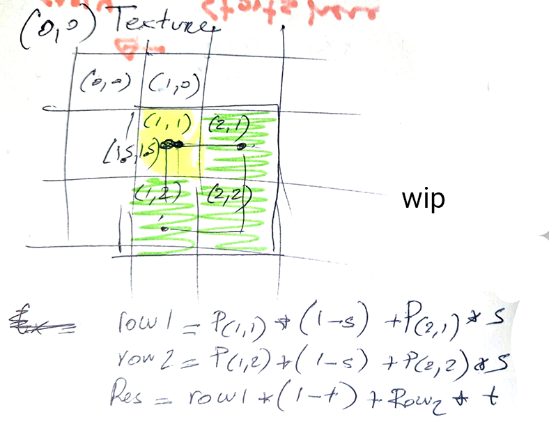
In the figure above we can see that our \(st\) or \(uv\) values are \{1.5,1.5}\) that is it's located in the center of the pixel located on on the second row and column of hte trexture, that is pixel with coordinates \{(1,1}\). With bilinear filtering (the linear mode) we will use the three adjecent pixels to that one pixel (in green in the image) forming a 2x2 pixels block where the pixel in the top-left corner contains the point we will be sampling from (sometimes refer to as the anchor point). Then we use linear interpolation to interpolate the pixel's pairs \(P_{1,1}\)-\(P{2,1}\) and \(P_{2,1}\)-\(P{2,2}\) linearly using \(s\) as the parameter of interpolation and finally linear interpoalte these results using \(t\) this time around to get a final result. Again this is a typical bilinear interpolation process which you can find explained in the leson on interpolation.
XX code
xx

Now, it's not entirely true that bilinear filtering only slightly addresses the filtering issue. There is a case where this type of filtering is very useful, and people from the '90s who played video games before bilinear filtering was natively supported by hardware (GPUs) can attest to it. The benefit of using this type of filtering is most noticeable when, for example, the triangle you are rendering is small in texture space (or perhaps large, but the texture resolution is low, say 64x64 pixels) yet large on the screen. In other words, the triangle on the screen covers many pixels, but in texture space, it only covers a few texels, as shown in the figure below.
The problem with point sampling in this scenario is that a single texel from the texture ends up covering many pixels in the image, causing the surface of the triangle to look blocky—a problem that many video games suffered from until the late '90s. I'm not a GPU or graphics card historian/guru, but I believe the first card to accelerate bilinear filtering via hardware was part of the Voodoo family, notably the Voodoo2 chips, which were released in the late '90s. A similar kind of problem occurs when several texels fit within a single pixel. This issue becomes more apparent when animation is involved (e.g., when the camera moves), as the "texels" on the screen seem to jump around from frame to frame, as seen in this clip.
In this scenario, in frame N, the pixel might sample a red texel in the texture, and in frame N+1, it might sample the texel right next to it, even though the triangle moves only slightly in relation to the camera. If this sample is very different in color or brightness, it will cause a noticeable jump.
Bilinear filtering helps in both cases, but it is especially effective in the first case (when one texel covers several pixels on the screen) as it creates a smooth transition from texel to texel, helping to reduce the blocky appearance. For the second case, bilinear filtering helps a little, but not completely, because this scenario is more directly related to the topic we will study in the next chapter, which deals with texture under-sampling. Addressing this issue requires more than just using a bilinear filter.
xx