Building a Basic Perspective Projection Matrix
Reading time: 21 mins.Understanding the Perspective Projection Matrix
A note of caution. The matrix introduced in this section is distinct from the projection matrices utilized in APIs like OpenGL, Direct3D, Vulkan, Metal or WebGL, yet it effectively achieves the same outcome. From the lesson 3D Viewing: the Pinhole Camera Model, we learned to determine screen coordinates (left, right, top, and bottom) using the camera's near clipping plane and angle-of-view, based on the specifications of a physically based camera model. These coordinates were then used to ascertain if the projected points fell within the visible image frame. In the lesson Rasterization: a Practical Implementation, we explored remapping the projected points' coordinates to NDC (Normalized Device Coordinates) space, using the screen coordinates to avoid direct comparison with the projected point coordinates by standardizing them within the [-1,1] range.
In this discussion, our approach deviates slightly. We start by presuming screen coordinates of (-1,1) for both left and right, and similarly for bottom and top (assuming a square screen), aligning with the desired range for coordinate comparison. Instead of scaling the projected point coordinates by the angle-of-view to map them to NDC space, we'll adjust the projected point coordinates directly to account for the camera's field-of-view. Both methodologies ultimately yield the same result.
Referencing our Geometry lesson, the equation for multiplying a point by a matrix is as follows:
$$ \begin{equation} \begin{bmatrix} x & y & z & w \end{bmatrix} * \begin{bmatrix} m_{00} & m_{01} & m_{02} & m_{03}\\ m_{10} & m_{11} & m_{12} & m_{13}\\ m_{20} & m_{21} & m_{22} & m_{23}\\ m_{30} & m_{31} & m_{32} & m_{33} \end{bmatrix} \end{equation} $$Resulting in the transformed coordinates:
$$ \begin{array}{l} x' = x * m_{00} + y * m_{10} + z * m_{20} + w * m_{30}\\ y' = x * m_{01} + y * m_{11} + z * m_{21} + w * m_{31}\\ z' = x * m_{02} + y * m_{12} + z * m_{22} + w * m_{32}\\ w' = x * m_{03} + y * m_{13} + z * m_{23} + w * m_{33} \end{array} $$Recall, the projection of point P onto the image plane, denoted as P', is obtained by dividing P's x- and y-coordinates by the inverse of P's z-coordinate:
$$ \begin{array}{l} P'_x=\dfrac{P_x}{-P_z} \\ P'_y=\dfrac{P_y}{-P_z} \\ \end{array} $$Now, how can we achieve the computation of P' through a point-matrix multiplication process?
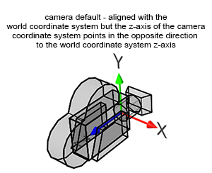
First, the coordinates \(x'\), \(y'\), and \(z'\) (of point \(P'\)) in the equation above need to be set as \(x\), \(y\), and \(-z\) respectively, where \(x\), \(y\), and \(z\) are the coordinates of point \(P\) that we want to project. Setting \(z'\) to \(-z\) instead of just \(z\) is crucial because, in the transformation from world space to camera space, all points defined in the camera coordinate system and located in front of the camera have a negative \(z\)-value. This is due to cameras typically pointing down the negative \(z\)-axis (Figure 1). Consequently, we assign \(z\) to \(z'\) but invert its sign so that \(z'\) becomes positive:
$$ \begin{array}{l} x' = x,\\ y' = y,\\ z' = -z \:\:\: \text{such that} \:\:\: z' > 0.\\ \end{array} $$Suppose, during the point-matrix multiplication process, we could divide \(x'\), \(y'\), and \(z'\) by \(-z\), resulting in:
$$ \begin{array}{l} x' = \dfrac {x}{-z},\\ y' = \dfrac {y}{-z},\\ z' = \dfrac {-z}{-z} = 1.\\ \end{array} $$These equations compute the projected coordinates of point \(P'\) (without worrying about \(z'\) for the moment). The next question is whether it's possible to achieve this result through point-matrix multiplication and what the corresponding matrix would look like. Initially, we establish the coordinates \(x'\), \(y'\), and \(z'\) as \(x\), \(y\), and \(-z\) respectively, which can be achieved using an identity matrix with slight modification:
$$ \begin{equation} \begin{bmatrix} x & y & z & (w=1) \end{bmatrix} * \begin{bmatrix} 1 & 0 & 0 & 0\\ 0 & 1 & 0 & 0\\ 0 & 0 & -1 & 0\\ 0 & 0 & 0 & 1\\ \end{bmatrix} \end{equation} $$ $$ \begin{array}{l} x' = x \cdot 1 + y \cdot 0 + z \cdot 0 + w \cdot 0 = x,\\ y' = x \cdot 0 + y \cdot 1 + z \cdot 0 + w \cdot 0 = y,\\ z' = x \cdot 0 + y \cdot 0 + z \cdot -1 + w \cdot 0 = -z,\\ w' = x \cdot 0 + y \cdot 0 + z \cdot 0 + (w=1) \cdot 1 = 1.\\ \end{array} $$The multiplication involves a point with homogeneous coordinates, where the fourth coordinate, \(w\), is set to 1. To convert back to Cartesian coordinates, \(x'\), \(y'\), and \(z'\) need to be divided by \(w'\):
... the homogeneous point \([x, y, z, w]\) corresponds to the three-dimensional Cartesian point \([x/w, y/w, z/w]\).
If \(w'\) equaled \(-z\), dividing \(x'\), \(y'\), and \(z'\) by \(-z\) would yield the desired result:
The key is utilizing the conversion from homogeneous to Cartesian coordinates in the point-matrix multiplication process to perform the perspective divide (dividing \(x\) and \(y\) by \(z\) to compute the projected coordinates \(x'\) and \(y'\)). This necessitates setting \(-z\) to \(w'\).
Can the perspective projection matrix be adjusted to ensure the point-matrix multiplication sets \(w'\) to \(-z\)? Observing the equation for \(w'\) reveals:
$$ \begin{array}{l} w' = x \cdot m_{03} + y \cdot m_{13} + z \cdot m_{23} + w \cdot m_{33} \end{array} $$With the point \(P\) \(w\)-coordinate equal to 1, this simplifies to:
$$ \begin{array}{l} w' = x \cdot m_{03} + y \cdot m_{13} + \color{red}{z \cdot m_{23}} + 1 \cdot m_{33} \end{array} $$The goal is for \(w'\) to equal \(-z\), achievable by setting the matrix coefficient \(m_{23}\) to \(-1\) and the others to 0, leading to:
$$w' = x \cdot 0 + y \cdot 0 + \color{red}{z \cdot -1} + 1 \cdot 0 = -z$$Thus, for \(w'\) to equal \(-z\), the matrix coefficients \(m_{03}\), \(m_{13}\), \(\color{red}{m_{23}}\), and \(m_{33}\) must be 0, 0, -1, and 0 respectively. Here is the updated perspective projection matrix:
$$ \left[ \begin{array}{rrrr}x & y & z & 1\end{array} \right] * \left[ \begin{array}{rrrr} 1 & 0 & 0 & 0\\ 0 & 1 & 0 & 0\\ 0 & 0 & -1 & \color{red}{-1}\\ 0 & 0 & 0 & 0 \end{array} \right] $$The significance here is in distinguishing between our specialized projection matrix and a standard affine transformation matrix. Normally, an affine transformation matrix's fourth column coefficients are set to \(\{0, 0, 0, 1\}\), as shown:
$$ \begin{bmatrix} \color{green}{m_{00}} & \color{green}{m_{01}} & \color{green}{m_{02}} & \color{blue}{0}\\ \color{green}{m_{10}} & \color{green}{m_{11}} & \color{green}{m_{12}} & \color{blue}{0}\\ \color{green}{m_{20}} & \color{green}{m_{21}} & \color{green}{m_{22}} & \color{blue}{0}\\ \color{red}{T_x} & \color{red}{T_y} & \color{red}{T_z} & \color{blue}{1}\\ \end{bmatrix} $$However, in our adjusted projection matrix, these coefficients are instead set to \(\{0, 0, -1, 0\}\):
$$ \left[ \begin{array}{ccc|r} \textcolor{green}{m_{00}} & \textcolor{green}{m_{01}} & \textcolor{green}{m_{02}} & \textcolor{blue}{0} \\ \textcolor{green}{m_{10}} & \textcolor{green}{m_{11}} & \textcolor{green}{m_{12}} & \textcolor{blue}{0} \\ \textcolor{green}{m_{20}} & \textcolor{green}{m_{21}} & \textcolor{green}{m_{22}} & \textcolor{blue}{-1} \\ \textcolor{red}{T_x} & \textcolor{red}{T_y} & \textcolor{red}{T_z} & \textcolor{blue}{0} \\ \end{array} \right] $$This modification ensures \(w'\) is set to \(-z\). If \(-z\) differs from 1, it necessitates the normalization of the coefficients of the transformed points. This process is essentially the perspective divide occurring when a point is multiplied by a projection matrix, highlighting the critical nature of this understanding.
When utilizing the specialized projection matrix in point-matrix multiplication, the resultant expressions for \(x'\), \(y'\), \(z'\), and \(w'\) are:
$$ \begin{array}{ll} x' = x \cdot 1 + y \cdot 0 + z \cdot 0 + 1 \cdot 0 & = & x,\\ y' = x \cdot 0 + y \cdot 1 + z \cdot 0 + 1 \cdot 0 & = & y,\\ z' = x \cdot 0 + y \cdot 0 + z \cdot -1 + 1 \cdot 0 & = & -z,\\ w' = x \cdot 0 + y \cdot 0 + z \cdot -1 + 1 \cdot 0 & = & -z. \end{array} $$Subsequent division of all coordinates by \(w'\) converts the point's homogeneous coordinates back to Cartesian coordinates:
$$ \begin{array}{ll} x' = \dfrac{x}{w'=-z},\\ y' = \dfrac{y}{w'=-z},\\ z' = \dfrac{-z}{w'=-z} = 1. \end{array} $$This process effectively achieves the desired outcome, aligning with the perspective projection principles. The next steps involve adjusting the projection matrix further to accommodate additional aspects of a realistic camera model, specifically:
1. Remapping \(z'\) within the range \([0,1]\): This adjustment is crucial for depth calculations in a 3D scene, ensuring that objects are correctly rendered with respect to their distance from the camera. It utilizes the camera's near (\(z_{near}\)) and far (\(z_{far}\)) clipping planes to linearly interpolate \(z'\) values within this range. The transformation is generally achieved through additional matrix operations that scale and translate \(z'\) values accordingly.
2. Incorporating the Camera's Angle of View: The field of view (FOV) parameter influences how much of the scene is visible through the camera, mimicking the effect of a pinhole camera model. This aspect is accounted for by adjusting the projection matrix to alter the scale of the projected points, thereby affecting the perceived FOV. The matrix adjustments typically involve scaling factors derived from the FOV, ensuring that the scene's spatial dimensions are correctly projected onto the 2D view space.
Remapping the Z-Coordinate
The normalization of the z-coordinate, scaling it between 0 and 1, is a critical step in the perspective projection process, as it ensures that objects are correctly rendered according to their distance from the camera. This scaling uses the camera's near and far clipping planes. The aim is to adjust the z-coordinate so that when a point lies on the near clipping plane, its transformed z-coordinate (\(z'\)) equals 0, and when it lies on the far clipping plane, \(z'\) equals 1. This is achieved by setting specific coefficients in the perspective projection matrix:
$$z' = x \cdot m_{20} + y \cdot m_{21} + z \cdot \color{green}{m_{22}} + 1 \cdot \color{red}{m_{23}}$$To fulfill the conditions for \(z'\) to be 0 at the near clipping plane and 1 at the far clipping plane, the coefficients for \(m_{22}\) and \(m_{23}\) are set as follows:
$$-\dfrac{f}{(f-n)},$$and
$$-\dfrac{f \cdot n}{(f-n)}$$respectively, where \(n\) is the distance to the near clipping plane and \(f\) is the distance to the far clipping plane. These adjustments ensure that \(z'\) is correctly normalized across the specified range.
When evaluating \(z'\) at the near and far clipping planes, with \(m_{20}\) and \(m_{21}\) set to 0, the results validate the effectiveness of these coefficients:
-
At the near clipping plane (\(z = n\)):
-
At the far clipping plane (\(z = f\)):
This demonstrates how the chosen coefficients correctly map \(z\) values at the near and far clipping planes to \(z'\) values of 0 and 1, respectively.
The resulting perspective projection matrix, incorporating these adjustments for \(z'\) normalization, is:
$$ \left[\begin{array}{cccc} 1 & 0 & 0 & 0 \\ 0 & 1 & 0 & 0 \\ 0 & 0 & -\dfrac{f}{(f-n)} & -1\\ 0 & 0 & -\dfrac{f \cdot n}{(f-n)} & 0\\ \end{array}\right] $$This matrix now not only projects points from 3D space to 2D space but also remaps their z-coordinates to a normalized range of [0,1], ensuring depth values are correctly interpreted for rendering.
Regarding the depth precision and the impact of the near and far clipping planes, it's important to note that the depth precision is not linear across this range. The precision is higher closer to the near clipping plane and decreases with distance. This non-linear distribution can lead to z-fighting, especially when the [near:far] range is excessively large. Thus, it's crucial to keep this range as tight as possible to mitigate depth buffer precision issues.
Taking the Field-of-View into Account
In this chapter, we assume the screen is square and the distance between the screen and the eye is equal to 1 to simplify the demonstration. A more generic solution will be provided in the next chapter.
To get a basic perspective projection matrix working, we need to account for the angle of view or field-of-view (FOV) of the camera. Changing the focal length of a zoom lens on a real camera alters the extent of the scene we see. We aim for our CG camera to function similarly.
The projection window size is [-1:1] in each dimension, meaning a projected point is visible if its x- and y-coordinates are within this range. Points outside this range are invisible and not drawn.
Note that in our system, the screen window's maximum and minimum values remain unchanged, always in the range [-1:1], assuming the screen is square. When points' coordinates are within the range [-1,1], we say they are defined in NDC space.
Remember from chapter 1, the goal of the perspective projection matrix is to project a point onto the screen and remap their coordinates to the range [-1,1] (or to NDC space).
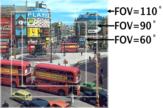
The distance to the screen window from the eye position remains the same (equal to 1). However, when the FOV changes, the screen window should become larger or smaller accordingly (see figures 2 and 5). How do we reconcile this contradiction? Since we want the screen window size to remain fixed, we instead adjust the projected coordinates by scaling them up or down, testing them against the fixed borders of the screen window. Let's explore a few examples.
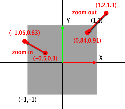
Imagine a point whose projected x-y coordinates are (1.2, 1.3). These coordinates are outside the range [-1:1], making the point invisible. If we scale them down by multiplying them by 0.7, the new, scaled coordinates become (0.84, 0.91), making the point visible as both coordinates are now within the range [-1:1]. This action is analogous to zooming out, which means decreasing the focal length on a zoom lens or increasing the FOV. Conversely, to achieve the opposite effect, multiply by a value greater than 1. For instance, a point with projected coordinates (-0.5, 0.3) scaled by 2.1 results in new coordinates (-1.05, 0.63). The y-coordinate remains within the range [-1:1], but the x-coordinate is now lower than -1, rendering the point invisible. This effect is akin to zooming in.
To scale the projected coordinates, we use the camera's field of view. The FOV intuitively controls how much of the scene is visible. For more information, see the lesson 3D Viewing: the Pinhole Camera Model.
The FOV can be either the horizontal or vertical angle. If the screen is square, the choice of FOV does not matter, as all angles are the same. However, if the frame's aspect ratio differs from 1, the choice of FOV becomes significant (refer to the lesson on cameras in the basic section). In OpenGL (GLUT, more precisely), the FOV corresponds to the vertical angle. In this lesson, the FOV is considered to be the horizontal angle (as is also the case in Maya).
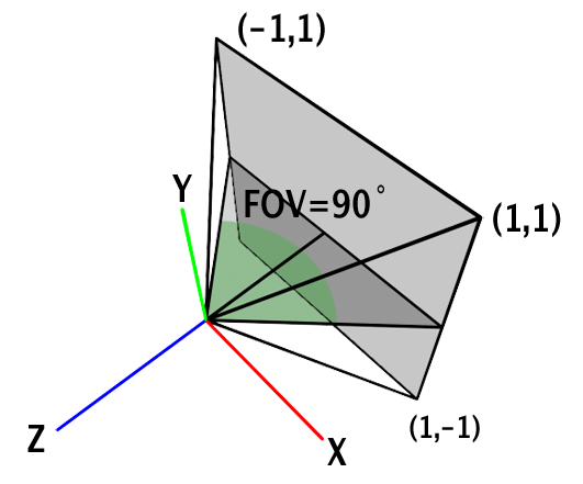
The value of the field-of-view (FOV) is not utilized directly in calculations; instead, the tangent of the angle is used. In computer graphics literature, the FOV can be defined either as the entire angle or half of the angle subtended by the viewing cone. It is more intuitive to perceive the FOV as the angular extent of the visible scene rather than half of this angle, as illustrated in figures 3 and 5. However, to derive a value for scaling the projected coordinates, the FOV angle needs to be halved. This is why the FOV is sometimes expressed as the half-angle.
The rationale behind dividing the angle by two lies in focusing on the right triangle within the viewing cone. The angle between the hypotenuse and the adjacent side of the triangle, or the FOV half-angle, dictates the length of the triangle's opposite side. Altering this angle allows for the scaling of the image window's border. Utilizing the tangent of this angle scales our projected coordinates. Notably, at an FOV half-angle of 45 degrees (total FOV of 90 degrees), the tangent of the angle equals 1, leaving the coordinates unchanged when multiplied by this value. For FOV values less than 90 degrees, the tangent of the half-angle yields values smaller than 1, and for values greater than 90 degrees, it results in values greater than 1.
However, the required effect is the inverse. Zooming in, which corresponds to a decrease in FOV, necessitates multiplying the projected point coordinates by a value greater than 1. Conversely, zooming out, which increases the FOV, requires multiplication by a value less than 1. Therefore, the reciprocal of the tangent, or one over the tangent of the FOV half-angle, is employed.
The final equation to compute the scaling factor for the projected point coordinates is as follows:
$$S = \dfrac{1}{\tan(\dfrac{fov}{2}*\dfrac{\pi}{180})}$$With this scaling factor, the complete version of our basic perspective projection matrix is:
$$ \left[\begin{array}{cccc} S & 0 & 0 & 0 \\ 0 & S & 0 & 0 \\ 0 & 0 & -\dfrac{f}{(f-n)} & -1\\ 0 & 0 & -\dfrac{f \cdot n}{(f-n)} & 0\\ \end{array}\right] $$This matrix accounts for the FOV by scaling the x and y coordinates of projected points, thus effectively incorporating the angle of view into the perspective projection process.
Are There Different Ways of Building this Matrix?
Yes and no. Some renderers may implement the perspective projection matrix differently. For instance, OpenGL utilizes a function called glFrustum to create perspective projection matrices. This function accepts arguments for the left, right, bottom, and top coordinates, in addition to the near and far clipping planes. Unlike our approach, OpenGL projects points onto the near-clipping plane, rather than onto a plane one unit away from the camera position. The matrix configuration might also appear slightly different.
It's important to pay attention to the convention used for vectors and matrices. The projected point can be represented as either a row or column vector. Additionally, it's crucial to verify whether the renderer employs a left- or right-handed coordinate system, as this could alter the sign of the matrix coefficients.
Despite these variations, the fundamental concept of the perspective projection matrix remains consistent across all renderers. They invariably divide the x- and y-coordinates of a point by its z-coordinate. Ultimately, all matrices are designed to project the same points to the same pixel coordinates, regardless of the specific conventions or the matrix being used.
We will explore the construction of the OpenGL matrix in greater detail in the next chapter.
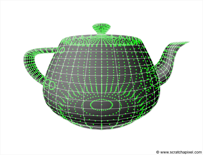
Test Program
To validate our basic perspective projection matrix, we developed a simple program to project the vertices of a polygonal object (Newell's teapot) onto the image plane using the projection matrix crafted in this chapter. The program is straightforward. It employs a function to construct the perspective projection matrix based on the camera's near and far clipping planes and the camera field-of-view, specified in degrees. The teapot's vertices are stored in an array. Each point undergoes projection onto the image plane via straightforward point-matrix multiplication, initially transforming points from world or object space to camera space. The function multPointMatrix facilitates the multiplication of a point by a matrix, highlighting the creation of the fourth component, \(w\), and dividing the resultant point's coordinates by \(w\) if \(w\) differs from 1—this stage marks the perspective or \(z\) divide. A point is deemed visible only if its projected \(x\) and \(y\) coordinates fall within the \([-1:1]\) interval, irrespective of the image's aspect ratio. Points outside this range are considered beyond the camera's screen boundaries. Visible points are then mapped to raster space, i.e., pixel coordinates, through a remapping from \([-1:1]\) to \([0:1]\), followed by scaling to the image size and rounding to the nearest integer to align with pixel coordinates.
#include <cstdio>
#include <cstdlib>
#include <fstream>
#include "geometry.h"
#include "vertexdata.h"

void setProjectionMatrix(const float &angleOfView, const float &near, const float &far, Matrix44f &M)
{
    // set the basic projection matrix
    float scale = 1 / tan(angleOfView * 0.5 * M_PI / 180);
    M[0][0] = scale;  // scale the x coordinates of the projected point
    M[1][1] = scale;  // scale the y coordinates of the projected point
    M[2][2] = -far / (far - near);  // used to remap z to [0,1]
    M[3][2] = -far * near / (far - near);  // used to remap z [0,1]
    M[2][3] = -1;  // set w = -z
    M[3][3] = 0;
}

void multPointMatrix(const Vec3f &in, Vec3f &out, const Matrix44f &M)
{
    //out = in * M;
    out.x   = in.x * M[0][0] + in.y * M[1][0] + in.z * M[2][0] + M[3][0];
    out.y   = in.x * M[0][1] + in.y * M[1][1] + in.z * M[2][1] + M[3][1];
    out.z   = in.x * M[0][2] + in.y * M[1][2] + in.z * M[2][2] + M[3][2];
    float w = in.x * M[0][3] + in.y * M[1][3] + in.z * M[2][3] + M[3][3];

    // normalize if w is different than 1 (convert from homogeneous to Cartesian coordinates)
    if (w != 1) {
        out.x /= w;
        out.y /= w;
        out.z /= w;
    }
}

int main(int argc, char **argv)
{
    uint32_t imageWidth = 512, imageHeight = 512;
    Matrix44f Mproj;
    Matrix44f worldToCamera;
    worldToCamera[3][1] = -10;
    worldToCamera[3][2] = -20;
    float angleOfView = 90;
    float near = 0.1;
    float far = 100;
    setProjectionMatrix(angleOfView, near, far, Mproj);
    unsigned char *buffer = new unsigned char[imageWidth * imageHeight];
    memset(buffer, 0x0, imageWidth * imageHeight);
    for (uint32_t i = 0; i < numVertices; ++i) {
        Vec3f vertCamera, projectedVert;
        multPointMatrix(vertices[i], vertCamera, worldToCamera);
        multPointMatrix(vertCamera, projectedVert, Mproj);
        if (projectedVert.x < -1 || projectedVert.x > 1 || projectedVert.y < -1 || projectedVert.y > 1) continue;
        // convert to raster space and mark the position of the vertex in the image with a simple dot
        uint32_t x = std::min(imageWidth - 1, (uint32_t)((projectedVert.x + 1) * 0.5 * imageWidth));
        uint32_t y = std::min(imageHeight - 1, (uint32_t)((1 - (projectedVert.y + 1) * 0.5) * imageHeight));
        buffer[y * imageWidth + x] = 255;
    }
    // save to file
    std::ofstream ofs;
    ofs.open("./out.ppm");
    ofs << "P5\n" << imageWidth << " " << imageHeight << "\n255\n";
    ofs.write((char*)buffer, imageWidth * imageHeight);
    ofs.close();
    delete [] buffer;

    return 0;
}
Testing the program with the teapot rendered in a commercial renderer using identical camera settings resulted in matching images, as expected. The teapot geometry and program files are detailed in the Source Code chapter at the end of this lesson.
What's Next?
In the upcoming chapter, we'll delve into the construction of the perspective projection matrix as utilized in OpenGL. While the foundational principles remain consistent, OpenGL diverges by projecting points onto the near clipping plane and remapping the projected point coordinates to Normalized Device Coordinates (NDC) space. This remapping leverages screen coordinates derived from the camera's near clipping plane and angle-of-view, culminating in a distinct matrix configuration.
Following our exploration of the perspective projection matrix in OpenGL, we'll transition to discussing the orthographic projection matrix. Unlike its perspective counterpart, the orthographic projection matrix offers a different view of three-dimensional scenes by projecting objects onto the viewing plane without the depth distortion inherent in perspective projection. This makes it particularly useful for technical and engineering drawings where maintaining the true dimensions and proportions of objects is crucial.