Volume Rendering

Volume Rendering of a 3D Density Field

So far we have only learned how to render homogeneous volumetric objects. Objects whose scattering and absorption coefficients are constant through space. That's fine but a bit boring and not really how things look in nature. If you look at clouds of smoke coming out of steam trains these volumes are heterogeneous. Some parts are more opaque than others. So how do we render heterogeneous volume objects?

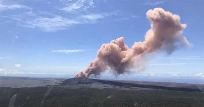
In the real world, we would say that the absorption or scattering coefficients are varying through space. The higher the absorption coefficient, the more opaque the volume. And the scattering and absorption could vary through space independently of each other. We generally choose a more practical approach though, which is to use a constant value for both the scattering and absorption coefficients for a given volumetric object and use the density parameter instead to modulate the volume's appearance through space. Imagine that the density parameter (which is just a real number like a float or a double in programming terms) varies through space. We can then do something like this:

Where \(\sigma_s'\) here is just the scattering coefficient modulated by the space-varying density parameter. The extinction coefficients \(\sigma_t\) used in the Beer's Law equation, which is the sum of the absorption and scattering coefficients, are also modulated by the space-varying density parameter. And \(density(p)\) is a kind of function that returns the density at point p in space. By doing so, we can produce images of volume objects such as the volcano smoke plume from the image above.

Now the question is how do we generate this density field? You can use two techniques:

1. Procedural: you can use a 3D texture such as the Perlin noise function to procedurally create a space-varying density field.

2. Simulation: you can use a fluid simulation program that simulates the motion of fluids (such as smoke) to generate a space-varying density field too.

In this chapter, we will use the first approach. In the next chapter, we will learn how to render the result of a fluid simulation.

Generating a density field using a noise function

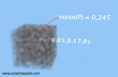
In this lesson, we will be using the Perlin noise function to generate a 3D density field procedurally. If you are unfamiliar with the concept of procedural noise generation we recommend that you read the following two lessons: Value Noise and Procedural Patterns (Part 1) and Perlin Noise (Part 2).

What is a procedural noise function (in this case the Perlin noise function)? It's a function (in the programmatic sense of the term) that procedurally generates a noise pattern through 3D space. We can use this pattern to generate a density field whose values vary through space. The noise function takes a point as an argument and returns the value of the 3D noise texture at that point (a real number like a float or a double). This value is bound to the range [-1,1]. Density can either be 0 (no volume) or positive so we will need to either clip or remap the values of the noise function to get positive values for the densities. In the following code snippet, we remap the values from [-1,1] to [0,1]:

float density = (noise(pSample) + 1) * 0.5;

Where pSample here is the position of a sample along the camera ray as we march through the volume.

For the noise function, we will be using the implementation of the improved Perlin noise provided by Ken Perlin himself (link). Again, you can learn how and why this code works in the lesson devoted to Perlin Noise (Part 2) if you are interested. But in this particular lesson, we will assume that you are familiar with the function. If you don't, don't worry too much. All you need to care about is that you pass to the function the position of the point in 3D space where you want the function to be evaluated, and it returns for that point a value in the range [-1,1]. Here is the code for reference (check the file provided in the source code section to get the full implementation):

int p[512]; // permutation table (see source code)
 
double fade(double t) { return t * t * t * (t * (t * 6 - 15) + 10); }
double lerp(double t, double a, double b) { return a + t * (b - a); }
double grad(int hash, double x, double y, double z)
{
    int h = hash & 15;
    double u = h<8 ? x : y,
           v = h<4 ? y : h==12||h==14 ? x : z;
    return ((h&1) == 0 ? u : -u) + ((h&2) == 0 ? v : -v);
}
 
double noise(double x, double y, double z)
{
    int X = (int)floor(x) & 255,
        Y = (int)floor(y) & 255,
        Z = (int)floor(z) & 255;
    x -= floor(x);
    y -= floor(y);
    z -= floor(z);
    double u = fade(x),
           v = fade(y),
           w = fade(z);
    int A = p[X  ]+Y, AA = p[A]+Z, AB = p[A+1]+Z,
        B = p[X+1]+Y, BA = p[B]+Z, BB = p[B+1]+Z;
 
    return lerp(w, lerp(v, lerp(u, grad(p[AA  ], x  , y  , z   ),
                                   grad(p[BA  ], x-1, y  , z   )),
                           lerp(u, grad(p[AB  ], x  , y-1, z   ),
                                   grad(p[BB  ], x-1, y-1, z   ))),
                   lerp(v, lerp(u, grad(p[AA+1], x  , y  , z-1 ),
                                   grad(p[BA+1], x-1, y  , z-1 )),
                           lerp(u, grad(p[AB+1], x  , y-1, z-1 ),
                                   grad(p[BB+1], x-1, y-1, z-1 ))));
}

And finally, here is how we will be using it in our ray-marching program:

Color integrate(const Ray& ray, ...)
{
    float sigma_a = 0.1;
    float sigma_s = 0.1;
    float sigma_t = sigma_a + sigma_s;
    ...
    float transmission = 1; // fully transmissive to start with
    for (size_t n = 0; n < numSteps; ++n) {
        float t = tMin + stepSize * (n + 0.5);
        Point p = ray.orig + ray.dir * t;
        // density is no longer a constant value. It varies through space.
        <span style="color: red; font-weight: bold; background-color: rgba(255,0,0,0.1); border: 1px none rgba(255,0,0,0.3);">float density = (1 + noise(p)) / 2;</span>
        float sampleAtt = exp(-density * sigma_t * stepSize);
        // transmission is attenuated by sample opacity
        transmission *= samplAtt;
        ...
    }
}

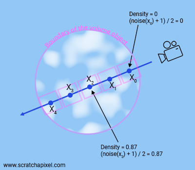
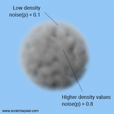
This is a rather simple change as you can see compared to the program we've been using to render homogeneous volume objects in the previous chapter. We move the declaration of the density variable inside the ray-marching loop which is no longer a constant value but is now a space-varying parameter. Figure 2 shows what's happening visually. We sample the density field as we march along the ray, where, once again, a noise function is used for the generation of that density field. For each sample along the ray, we evaluate the noise function using the sample position as the function input parameter and use the result as the value for the density at that point. Figure 3 shows the result applied to a volumetric sphere.

To be sure you understand what's going on here, we've plotted the noise function over some distance and the transmission value over the same distance using that same noise function for the density. The result is shown in the image below. We've also plotted how Beer's Lambert law would look like if that volume had a constant density (in green) vs a space-varying density. As you can see, the green curve (constant density) is perfectly smooth whereas the red curve (heterogeneous) is not. Note that transmission stays more or less constant where the noise function returns values closer to 0, whereas transmission drops sharply (the volume is denser) where the noise function is higher. All that is expected, but seeing it hopefully helps.

float stepSize = 1. / 51.2;
float sigma_t = 0.9;
float t = 0;
float Thomogeneous = 1;
float Theterogeneous = 1;
for (int x = 0; x < 512; x++, t += stepSize) {
    float noiseVal = powf((1 + noise(t, 0.625, 0)) / 2.f, 2);
    float samplAttHeterogeneous = exp(-noiseVal * stepSize * sigma_t);
    Theterogeneous *= samplAttHeterogeneous;
    float sampleAttHomogeneous = exp(-0.5 * stepSize * sigma_t);
    Thomogeneous *= sampleAttHomogeneous;
    fprintf(stderr, "%f %f %f\n", t, Theterogeneous, Thomogeneous);
}

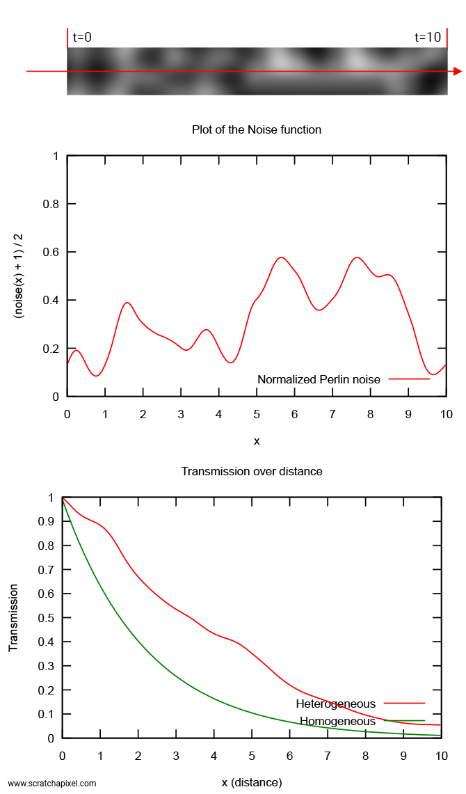
But there's a problem. This code works to compute the volume transmission value, but the code we've been using to calculate the in-scattering contribution (remember the Li term?) however will not as is. We will now explain why and what changes we need to make to get it to work with a heterogeneous participating medium.

In-scattering for a heterogenous participating medium

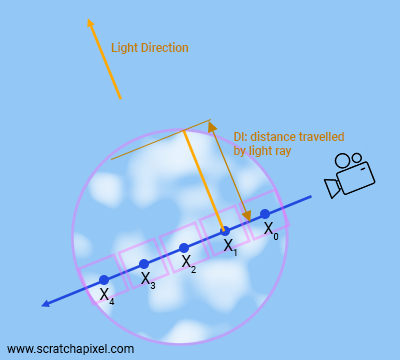
Hopefully, by looking at Figure 4, you should get a sense of what the problem is. For homogeneous volume objects, all we had to do when it came to light rays was to find the distance from the sample point to the boundary of the object in the direction of the light. Then apply Beer's Law using that distance (let's call it Dl) and the volume extinction coefficient (sigma_t = sigma_a + sigma_s) to find out how much light we are left with (how much is being transmitted) after it has traveled through the volume to the sample point. Easy:

Color lighRayContrib = exp(-Dl * sigma_t * density) * lightColor;

The problem with heterogeneous volumes is that this is no longer valid since density varies along the light rays as well which is visible in Figure 4. Be mindful: we are not solving the same problem as the problem we solved in chapter 2 with forward ray-marching. The reason why we used ray-marching so far, was to estimate the in-scattering term along the camera ray. Nothing else. However, the ray-marching technique will be useful here again to estimate the in-scattering term as well as estimate the camera and light rays transmission as they travel through a heterogeneous participating medium. Not the same problem (estimating the in-scattering vs estimating the transmission of the rays), though the same technique (forward ray-marching in this particular case, which is a form of stochastic sampling method). We need to break the ray into a series of segments, and estimate the transmission of each one of the segments, assuming that over the segment's length (within the small volume element defined by step size), the density of the volume element is uniform, and then multiply the total transmission value by the sample's transmission as we move along the ray. In pseudo-code, this could be implemented as follows:

// compute light ray transmission in heterogeneous medium
float transmission = 1;
float stepSize = Dl / numSteps;
for (n = 0; n < numSteps; ++n) {
    float t = stepSize * (n + 0.5);
    float sampleAtt = exp(-density(evalDensity(t) * stepSize * sigma_t);
    transmission *= samplAtt;
}

Compare this code with the code we used in the previous chapters to calculate the value of the camera ray transmission value as we march along the ray from t0 to t1.

float sigma_t = sigma_a + sigma_s;
float density = 0.1; // density is constant. Used to scale sigma_t
float transparency = 1; // initialize transparency to 1 
 
for (int n = 0; n < ns; ++n) { 
    float t = isect.t1 - step_size * (n + 0.5); 
    vec3 sample_pos= ray_orig + t * ray_dir; // sample position (middle of the step) 
 
<span style="display: block; color: red; font-weight: bold; background-color: rgba(255,0,0,0.1); border: 1px none rgba(255,0,0,0.3);">    // compute sample transparency using Beer's law
    float sample_transparency = exp(-step_size * sigma_t * density); 
 
    // attenuate global transparency by sample transparency
    transparency *= sample_transparency; 
</span>
    // In-scattering. 
    if (hitObject->intersect(sample_pos, light_dir, isect_vol) && isect_vol.inside) { 
        ...
        result += ... 
    } 
 
    // finally attenuate the result by sample transparency
    result *= sample_transparency; 
}

The two code snippets are doing the same thing. There's one little mathematical trick we can take advantage of which we haven't spoken about until now (because precisely now is a good time to do so). Here it is:

If you look at the code, you can see that the transmission value is essentially a series of exponentials multiplied by each other. If you unfold the ray-marching loop (snippet 2) you get something like this:

// dx = stepSize, and noise(x) is in the range [0,1]
float t0 = dx * (0.5); // n = 0
float t1 = dx * (1 + 0.5); // n = 1
float t2 = dx * (2 + 0.5); // n = 2
...
float transmission = exp(-dx * sigma_t * noise(t0)) *  
                     exp(-dx * sigma_t * noise(t1)) * 
                     exp(-dx * sigma_t * noise(t2)) * 
                     ...;

If we re-write this code using the mathematical property of exponentials we just learned about, we get:

float tau = noise(t0) + noise(t1) + noise(t2) + ...;
float transmission = exp(-tau * sigma_t * dx);

In other words, as we march along the light ray (exactly like we do for camera rays), all we need to do is accumulate the density values at each sample along the ray, then use this sum to calculate the light ray attenuation/transmission value in a single call to the exponential function (which is a bit of a time saver indeed). This concept is illustrated in the image below.

float transmission = 1; // set the camera ray transmission value (full transmission)
vec3 result = 0; // the camera ray radiance (light energy traveling from the volume to the eye)
for (n = 0; n < numSteps; ++n) {
    float t = t0 + stepSize * (n + 0.5);
    vec3 samplePos = ray.orig + t * ray.dir;
    float sampleDensity = evalDensity(samplePos);
    // we need this intermediate result to attenuate the Li term (see below)
    transmission *= exp(-sampleDensity * sigma_t * stepSize);
    // inscattering (Li(x))
    if (density > 0 && hit_object->intersect(...) {
        float tau = 0;
        for (nl = 0;  nl < numStepsLight; ++nl) {
            float tLight = stepSize * (nl + 0.5);
            vec samplePosLight = samplePos + tLight * lightDirection;
            tau += evalDensity(samplePosLight);
        }
        // calculate light ray transmission value at the very end
        float lightRayAtt = exp(-tau * sigma_t * stepSize);
        result += lightColor * lightRayAtt * sigma_s * ... * transmission;
    }
}

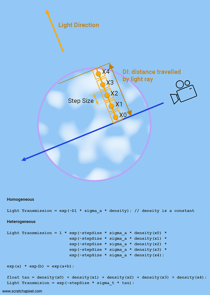
The name "tau" is not chosen by mistake. You will often see it being used in the literature to denote a quantity called the optical depth. Two Greek letters are often used for this quantity: either tau (\(\tau\)) or rho (\(\rho\)). We won't give a formal definition of what the optical depth is in this chapter, as this might be confusing at this point. But we do in the chapter Volume Rendering: Summary, Equations / Theory.

That's it! Now you have everything you need to render an accurate image of heterogeneous volume objects. This last figure shows what the transmission curve looks like for a given noise profile.

Practical (and functional) implementation

Let's make the necessary adjustments to our program to demonstrate how this would work in practice. Remember that the algorithm now works as follows:

1. Ray-march along the camera ray. At each sample along the camera ray, estimate the density at the sample location to calculate the sample transmission and estimate the in-scattering contribution.

2. Ray-march along light rays: whereas before we only marched along camera rays, we now need to ray-march along light rays too. For homogeneous volume objects, we only needed to march along the camera rays to estimate the in-scattering term. Whereas for heterogeneous, we need to do so along the camera rays to estimate the in-scattering term (this doesn't change) but now also to evaluate the density term along the ray. And we need to ray-march along the light rays to evaluate the density function along these rays as well.

In other words, we need to ray march along both the camera and the light rays now, and evaluate at each sample along these rays a density function. Currently the Perlin noise function. This is a lot of operations, and as you will see rendering our sphere as a heterogeneous medium will take significantly longer than its homogeneous counterpart.

// [comment]
// This function is now called by the integrate function to evaluate the density of the 
// heterogeneous volume sphere at sample position p. It returns the value of the Perlin noise
// function at that 3D position remapped to the range [0,1]
// [/comment]
float eval_density(const vec3& p)
{ 
    float freq = 1;
    return (1 + noise(p.x * freq, p.y * freq, p.z * freq)) * 0.5;
}

vec3 integrate(
    const vec3& ray_orig, 
    const vec3& ray_dir, 
    const std::vector<std::unique_ptr<Sphere>>& spheres)
{
    ...

    const float step_size = 0.1;
    float sigma_a = 0.5; // absorption coefficient
    float sigma_s = 0.5; // scattering coefficient
    float sigma_t = sigma_a + sigma_s; // extinction coefficient
    float g = 0; // henyey-greenstein asymetry factor
    uint8_t d = 2; // russian roulette "probability"

    int ns = std::ceil((isect.t1 - isect.t0) / step_size);
    float stride = (isect.t1 - isect.t0) / ns;

    vec3 light_dir{ -0.315798, 0.719361, 0.618702 };
    vec3 light_color{ 20, 20, 20 };

    float transparency = 1; // initialize transmission to 1 (fully transparent)
    vec3 result{ 0 }; // initialize volumetric sphere color to 0

    // The main ray-marching loop (forward, march from t0 to t1)
    for (int n = 0; n < ns; ++n) {
        // Jittering the sample position
        float t = isect.t0 + stride * (n + distribution(generator));
        vec3 sample_pos = ray_orig + t * ray_dir;

        // [comment]
        // Evaluate the density at the sample location (space varying density)
        // [/comment] float eval_density(const vec3& p)
        <span style="color: red; font-weight: bold; background-color: rgba(255,0,0,0.1); border: 1px none rgba(255,0,0,0.3);">float density = eval_density(sample_pos);</span>
        float sample_attenuation = exp(-step_size * density * sigma_t);
        transparency *= sample_attenuation;

        // In-scattering.
        IsectData isect_light_ray;
        if (density > 0 && 
            hit_sphere->intersect(sample_pos, light_dir, isect_light_ray) && 
            isect_light_ray.inside) {
            size_t num_steps_light = std::ceil(isect_light_ray.t1 / step_size);
            float stide_light = isect_light_ray.t1 / num_steps_light;
            float tau = 0;
            // [comment]
            // Ray-march along the light ray. Store the density values in the tau variable.
            // [/comment] float eval_density(const vec3& p)
            for (size_t nl = 0; nl < num_steps_light; ++nl) {
                float t_light = stide_light * (nl + 0.5);
                vec3 light_sample_pos = sample_pos + light_dir * t_light;
                <span style="color: red; font-weight: bold; background-color: rgba(255,0,0,0.1); border: 1px none rgba(255,0,0,0.3);">tau += eval_density(light_sample_pos);</span>
            }
            float light_ray_att = exp(-tau * stide_light * sigma_t);
            result += light_color *       // light color
                      light_ray_att *     // light ray transmission value
                      phaseHG(-ray_orig, light_dir, g) * // phase function
                      sigma_s *           // scattering coefficient
                      transparency *      // ray current transmission value
                      stride *            // dx in our Riemann sum
                      density;            // volume density at the sample location
        }

        // Russian roulette
        if (transparency < 1e-3) {
            if (distribution(generator) > 1.f / d)
                break;
            else
                transparency *= d;
        }
    }

    // combine background color and volumetric sphere color
    return background_color * transparency + result;
}

In this implementation, the step size used for the camera and the light rays is the same. This doesn't need to be. To speed things up you can use a bigger step size to estimate the light rays transmission values. Also, now that we use a procedural texture we may encounter some filtering issues. If the frequency at which you sample the noise function is too low, you may miss some details from the procedural texture and you will eventually get aliasing issues. Again this is a filtering issue that we won't be digging into now but be aware that the step size, the noise frequency, and your image resolution are somehow interconnected (from a sampling point of view).

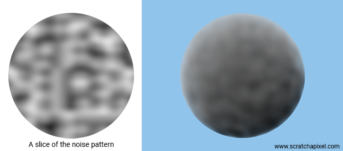
You might be surprised that the program output (right) doesn't look more like a cloud already. However, as you can see with an image of the noise pattern (left), the "lumps" making up the noise pattern are rather smooth by default which is why the volume has a smooth appearance as well. The art of making cloud-looking procedural noise requires tweaking the result of the noise function in different ways to get visually more interesting results (as we will show further down).

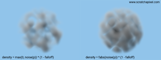
Here are a couple of simple variations you can already try: removing the negative values from the noise function (left) and taking the noise function's absolute value (right). The falloff parameter is explained further down.

However unspectacular, this is exactly the technique that was used to create the spectacular volumetric effects of the movie Contact's opening sequence (1997). These images were rendered using Pixar's renderer and created by Sony Picture Imageworks. This sequence was a huge technical undertaking at the time. As mentioned before, they used the same technique as the one provided in this lesson. The difference is that they used some geometry (and not basic spheres) to define the shape of the volumetric objects and some fractal patterns to give the nebulas a cloud-like texture. We will touch on the former technique in the last chapter of this lesson (volume rendering in production). As for a cloud-like texture, let's now see what we can do...

Playing with the density function (to create more interesting looks & animations)

Writing a ray-marcher is one thing. Creating a cloud-like procedural texture is another. Whereas the former is a science, the latter is more a matter of art: using a series of mathematical tools to shape the procedural texture and spending a lot of time tweaking the parameters until you eventually get something you are satisfied with. Our goal here is not to create convincing and wow images, but to give you the tools or bricks that first help you understand how things work and second, that you can eventually recombine yourself into more complex systems to make some "wow" images if you want to. But we will leave that up to you... Share them with us though if you create something cool!

Now here are a few tricks that you can use to create more interesting cloud-like "spheres". This is just a short selection of some of these tools.

Smoothstep

The smoothstep function is a function you are familiar with as we've been using it already for several things, including for the noise function. It creates a "smooth" transition between two values. Here is one possible implementation of the function:

float smoothstep(float lo, float hi, float x)
{
    float t = std::clamp((x - lo) / (hi - lo), 0.f, 1.f);
    return t * t * (3.0 - (2.0 * t));
}

We can use this function to create a falloff near the sphere boundary. To do so, we will make some changes to the eval_density function to pass as parameters to the function, the sphere center, and the radius. By doing so, we can compute a normalized distance from the sample position to the center of the sphere, and use this value to adjust the density of the sphere-like so:

float eval_density(const vec3& sample_pos, const vec3& sphere_center, const float& sphere_radius)
{
    vec3 vp = sample_pos - sphere_center;
    float dist = std::min(1.f, vp.length() / sphere_radius);
    float falloff = smoothstep(0.8, 1, dist); // smooth transition from 0 to 1 as distance goes from 0.1 to 1
    return (1 - falloff);
}

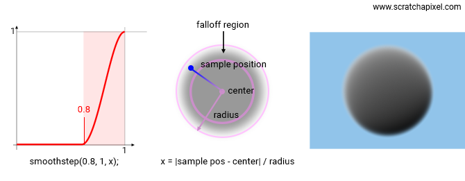
Again this technique is useful for fading out the volume before it reaches the boundary of the sphere. We use the smoothstep function to control how far from the edge or side the falloff begins (and eventually ends, but for a falloff effect, it should be kept to 1).

fBm

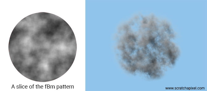
fBm (also known as plasma or "chaos" texture in the good old times) stands for Fractal Brownian Motion. In the field of computer graphics, it has a different meaning than in mathematics. We will be considering what it means for us, graphics engineers and artists. It's a kind of fractal pattern that is made out of a sum of procedural noise layers, whose frequency and amplitude vary from layer to layer. You can find some information on this pattern in the lessons from the Procedural Generation section.

The code of a typical fBm procedural texture can be constructed as follows:

float eval_density(const vec3& p, ...)
    vec3 vp = p - sphere_center;
    ...
    // build an fBm fractal pattern
    float frequency = 1;
    vp *= frequency; // scale the initial point value if necessary
    size_t numOctaves = 5; // number of layers
    float lacunarity = 2.f; // gap between successive frequencies
    float H = 0.4; // fractal increment parameter
    float value = 0; // result of the fBm (use this for our density)
    for (size_t i = 0; i < numOctaves; ++i) {
        value += noise(vp) * powf(lacunarity, -H * i);
        vp *= lacunarity;
    }

    // clip negative values
    return std::max(0.f, value) * (1 - falloff);
}

Building an fBm pattern takes two lines of code (looping over the layers). Many variations can be built from this basic version such as taking the noise function absolute value (a pattern known as turbulence) etc. Again check the procedural generation section if you want to learn more on this topic (and learn how to filter this pattern properly).

Bias

Bias shifts where the center (0.5) value will be while leaving 0 and 1 the same.

float eval_density(...) 
{
    float bias = 0.2;
    float exponent = (bias - 1.0) / (-bias - 1.0)
    // assuming exponent > 0
    return powf(noisePattern, exponent);
}

Rotate the noise pattern using the primitive local frame

Another technique was used a lot in the good old times (before fluid simulations became mainstream, thanks to an increase in computational power) to animate the noise pattern within the volume primitives (sphere, cubes, etc.). The sample position we pass to the density function is defined in world space, but we can define this point position within a system of reference that's attached to the sphere. In other words, we transform our sample point from world to object space. To define the sample point within the sphere reference system all we need to do is:

vec3 sample_object_space = sample_pos - center;

A more generic solution would consist of transforming the sphere primitive using matrices. Then we would be using the inverse of the object-to-world matrix to transform our sample point from world space to the sphere local reference system. However, we are not using matrices in our sample program for simplicity. But you can do this yourself easily with the information provided on Scratchapixel.

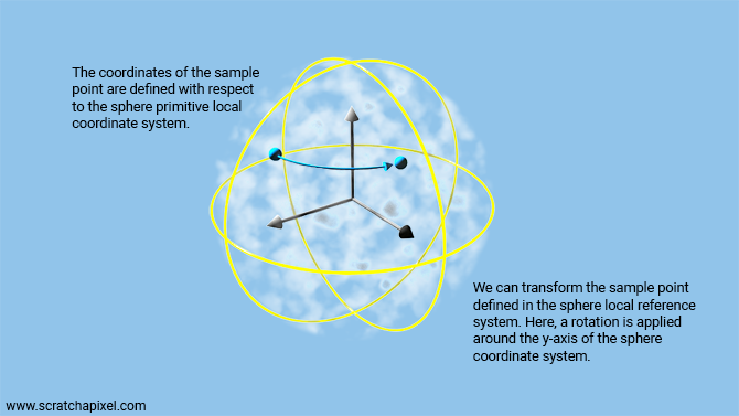
This technique is useful for the following reason: if we move the sphere, the coordinates of the point defined in the sphere's local frame of reference will not. And that can be used to insure that the noise pattern sticks with the sphere regardless of its transformation. Similar to the veins of a glass marble that you roll between your fingers. In the example we chose to illustrate this idea (even though it's a little different from what we just explained but the concept and the results are the same): we will be rotating the point in object space around the primitive sphere y-axis (a better solution would be to rate the sphere using an object-to-world matrix and then transform the sample point from world space to object space using the world-to-object matrix, but we were too lazy to do it here, so we decided to rotate the point in object space instead). As a result, we can see the fractal pattern rotating as well, again a little bit as if we were looking at a glass marble spinning. More sophisticated deformations (linear or not) can be applied using this method.

float eval_density(const vec3& p, const vec3& center, const float& radius)
{ 
    // transform the point from world to object space
    vec3 vp = p - center;
    vec3 vp_xform;

    // rotate our sample point in object space (frame is a global variable going from 1 to 120)
    float theta = (frame - 1) / 120.f * 2 * M_PI;
    vp_xform.x =  cos(theta) * vp.x + sin(theta) * vp.z;
    vp_xform.y = vp.y;
    vp_xform.z = -sin(theta) * vp.x + cos(theta) * vp.z;

    float dist = std::min(1.f, vp.length() / radius);
    float falloff = smoothstep(0.8, 1, dist);
    float freq = 0.5;
    size_t octaves = 5;
    float lacunarity = 2;
    float H = 0.4;
    vp_xform *= freq;
    float fbmResult = 0;
    float offset = 0.75;
    for (size_t k = 0; k < octaves; k++) {
        fbmResult += noise(vp_xform.x , vp_xform.y, vp_xform.z) * pow(lacunarity, -H * k);
        vp_xform *= lacunarity;
    }

    return std::max(0.f, fbmResult) * (1 - falloff);
}

Note how we can now clearly see the 3D structure of the fractal pattern.

And many more...

The list of "procedural" tricks can go on and on: displacement (we displace the edges of the volume using a noise function), different types of noise (billow, space-time which is an animated type of noise, etc.). We will eventually expand this list in a future revision of the lesson.

What did we learn so far?

See the last chapter for a summary of the techniques studied in this lesson.

Though what you can do now is use ray-marching to render single-scattering heterogeneous volumetric objects. And this is already a big accomplishment. Another thing that should be clear by now, is that with ray-marching, we break the volume object into smaller volume elements defined by the step size. This technique works because we assume that these tiny volume elements or samples are small enough to be homogeneous themselves. In short, you break down heterogeneous objects into small "bricks" which you can see as being "homogeneous". Though the bricks themselves can be different from one another. A little bit like when you build an object using Lego bricks.

Source code

The source code of a fully functional program implementing this technique is available in the source code section of this lesson. You can play with the eval_density() function to create different looks.