Volume Rendering Based On 3D Voxel Grids
Reading time: 33 mins.At the end of this chapter, you will be able to produce this sequence of images:
As mentioned in the previous chapter, you can create density fields using two techniques: procedurally or using fluid simulation software. In this chapter, we will look at the latter. Note that in this lesson, we won't learn how fluid simulation works. We will learn how to render the data produced from a fluid sim. We will learn about fluid simulation in the future, promise.
Step 1: Using a 3D Grid to Store Density Values
Many techniques for simulating a fluid (smoke, water, etc.) exist, but generally, at some point or another in the process, the result of the simulation is stored in a 3D grid. For simplicity and this lesson, we will assume that these grids have an equal resolution in all three dimensions (e.g. 32x32x32 in the x, y, and z coordinates respectively) and that this resolution is a power of 2 (8, 16, 32, 64, 128, etc.). This is just for the sake of this lesson. In practice, it doesn't have to be the case. Also, we won't be transforming the grid in this lesson. So we assume the grid is an axis-aligned box: we can treat our grid as an axis-aligned bounding box (AABB) which will simplify our ray-box intersection test. Making the solution generic (aka supporting grids that are not axis aligned can easily be done by transforming the camera ray into the grid object space using the grid's world-to-object transformation matrix as explained in this lesson).

Grids are nice to simulate the motion of fluids because, the grid's voxels (these are the small volume elements making up the grid which we can also call cells) are set with some initial density (imagine that they are filled up with smoke), and this density is distributed among the neighboring cells, as time progresses. The way they move from voxel to voxel is ruled by the Navier-Stokes equation. But again, this topic is left to another lesson. All you need to know for this lesson is that the results of fluid sims are stored in 3D grids made up of voxels that are storing density values (either 0 or a value greater than 0). Each voxel in the grid stores one unique density value (the density "filling up" the volume of the voxel). 3D Grids are too fluid sims, what bitmaps are to images. The density field is quantized. A 3D grid storing density values is rather simple to define in any programming language through they are subtleties that we will look into at the end of this chapter.
Besides the grid resolution (the number of voxels it contains in any dimension like 32x32x32), we also need to define the size of the grid in world space. That is the size of the object in the scene. We can do this in different ways, but for convenience, we will do so by defining the grid minimum and maximum bound or extent of the grid in world space like so: (-2,-2,2) and (2,2,2). Note that because our grid is a cube, for now, the values don't need to be symmetrical with respect to the world's origin however, the size of the grid in world space has to be the same in all three dimensions: e.g. (0.2,0.2,0.2), (10.2,10.2,10.2) is fine, (-1.2,2.2,3.2), (8.2,4.2,7.2) is not. Defining our grid world-space size that way is convenient, as the minimum and maximum extents can be plugged directly into the ray-box intersection routine (which we studied in the lesson A Minimal Ray-Tracer: Rendering Simple Shapes (Sphere, Cube, Disk, Plane, etc.)). So we already know how to compute the values for t0 and t1 for any ray that intersects a cube (similarly to the way we've done it for our sphere primitive).
You can modify the code from our previous chapters to render cubes instead of spheres. Let's also now use matrices to render the scene from a more interesting point of view. You should get something like this:
struct Grid {
    float *density;
    size_t dimension = 128;
    Point bounds[2] = { (-30,-30,-30), (30, 30, 30) };
};

bool rayBoxIntersect(const Ray& ray, const Point bounds[2], float& t0, float& t1)
{
    ...
    return true;
}

void integrate(const Ray& ray, const Grid& grid, Color& radiance, Color& transmission)
{
    Vector lightDir(-0.315798, 0.719361, 0.618702);
    Color lightColor(20);

    float t0, t1;
    if (rayBoxIntersect(ray, grid->bounds, t0, t1) {
        // ray march from t0 to t1

        radiance = ...;
        transmission = ...;
    }
}

Matrix cameraToWorld{ 0.844328, 0, -0.535827, 0, -0.170907, 0.947768, -0.269306, 0, 0.50784, 0.318959, 0.800227, 0, 83.292171, 45.137326, 126.430772, 1 };

int main()
{
    Grid grid;
    // allocate memory to read the data from the cache file
    size_t numVoxels = grid.resolution * grid.resolution * grid.resolution;
    // feel free to use a unique_ptr if you want to (the sample program does)
    grid.density = new float[numVoxels];
    std::ifstream cacheFile;
    cacheFile("./cache.0100.bin", std::ios::binary);
    // read the density values in memory
    cacheFile.read((char*)grid.density, sizeof(float) * numVoxels);

    Point origin(0);
    for (each pixel in the frame) {
        Vector rayDir = ...;
        Ray ray;
        ray.orig = origin * cameraToWorld;
        ray.dir = rayDir * cameraToWorld;

        Color radiance = 0, transmission = 1;
        integrate(ray, grid, radiance, transmission);

        pixelColor = radiance;
        pixelOpacity = 1 - transmission;
    }

    // free memory
    delete [] grid.density;
}
Don't worry too much about the content of the cache file for now. We will look into that later. But from the code above you should see that all we do is create a contiguous memory block to store as many float values as they are voxels in the grid. Then move the values from the disk to memory (line 36). Nothing fancy.
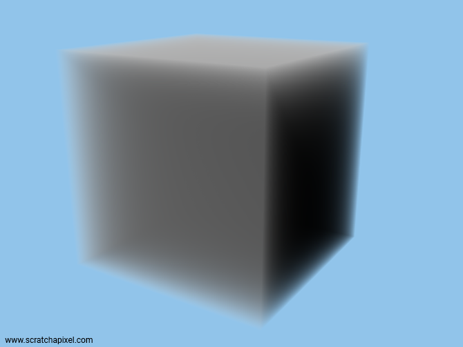
This is the image you should get. Now that we know that we will be using a 3D grid to store the density field values, that this grid has a resolution and a size, and that we know how to calculate the points where a ray intersects the box (aka the grid), let's see how we read the grid density values as we march along the ray.
Step 2: Ray-marching Through a Grid
Using a grid as an acceleration structure as explained in this lesson is quite involved. We have to find every single cell from the grid where the ray intersects to see if the geometry (triangles) that each of the intersected cells contains does intersect with the ray as well. While not super complicated this is not a super trivial task either (especially if you want to make it fast). So you might worry that we have to go through this process again. Well good news: not at all. With ray-marching, this is a trivial task since all we care about are the sample points along the ray as shown in the image below.
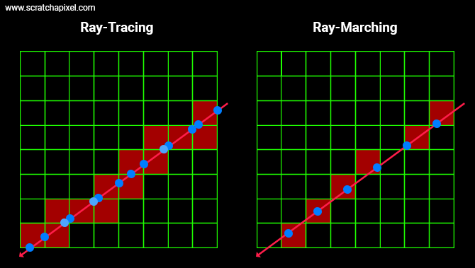
As we know the position of these points, all we are left with is to figure out the position of the voxel in the grid these points overlap (this is the topic of the next item) and read the density value stored in those voxels. No grid traversal is involved. Super simple. Now, let's see how we go from the sample point to the voxel's coordinates and read the value from memory using these coordinates.
Step 3: Reading the Density Values As We March Along The Ray
All we need to change from the code we used so far, is the evalDensity function. Instead of evaluating the density field defined by a procedural noise function at any given point in space, we will read the content of the grid at that position instead. That's a very small change. Everything else works the same. Normally we know that the sample point is always contained within the bounds of the grid (since it should be somewhere between the points where the ray interests the box). So this shouldn't be a problem though to make the code more robust, you probably still want to check the sample point coordinates against the grid's bounds, to prevent a crash.
Now, reading the density value from the grid can have different names. We generally call this a lookup. In OpenVDB, which is a library designed to efficiently store and read volume data, this is called probing (a rather uncommon name though). Okay, then how do we read the data?
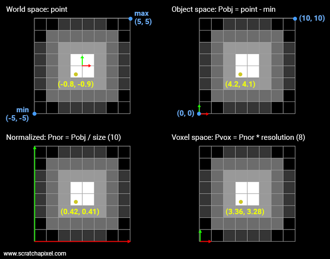
What we need to do is find a correspondence between the sample point and the voxel from the grid it falls into. The original sample point is defined in world space. So we need to convert that sample point to grid discrete coordinates. To do so we need to:
-
Transform the point from world space to object space. In our situation, all we need to do is remove from the sample position, the grid minimum extent. The sample point is now defined with respect to the "lower left" corner of the grid.
-
Then we need to divide the point in object space by the grid size (10 in our example). The point's coordinates are now normalized. We can speak of normalized coordinates (the coordinates of the point are contained in the range [0,1].
-
Finally, we need to multiply the normalized coordinates by the grid's resolution. We call this space the voxel space. At this point, the coordinates are still defined as floating numbers. To compute the grid coordinates and read the value for these coordinates from memory we need to round these floating numbers to the nearest integer. To prevent a crash, we need to be sure that the sample's coordinates in voxel space aren't greater than the grid resolution minus 1 (which can happen if any of the normalized coordinates is exactly 1). We can now read what the density value is at that position.
If you look at the (2D) example above, you can see that the point has coordinates (3.36, 3.28) in voxel space. From there we know that finding the index of the voxel in memory is just a matter of multiplying the integer part of the y-coordinate by 8 (the grid resolution) plus 3 (the integer part of the x-coordinate).
Here is the code:
float evalDensity(const Grid* grid, const Point& p)
{
    Vector gridSize = grid.bounds[1] - grid.bounds[0];
    Vector pLocal = (p - grid.bounds[0]) / gridSize;
    Vector pVoxel = pLocal * grid.baseResolution;

    int xi = static_cast<int>(std::floor(pVoxel.x));
    int yi = static_cast<int>(std::floor(pVoxel.y));
    int zi = static_cast<int>(std::floor(pVoxel.z));

    // nearest neighbor
    return grid->density[(zi * grid->resolution + yi) * grid->resolution + xi];
}
Here again (like for the Perlin noise function which has a similar need for converting points from world space to lattice space), we use the floor function, because if the normalized point's coordinates are lower than 0 (we will see why this can happen in a moment), we want the function to return 0 and not -1 (which a simple static_cast would eventually do).
We call this method the nearest-neighbor search interpolation because what you essentially do is retrieve the coordinates of the voxels the sample point falls into (as such it's not an interpolation). Other methods exist, though, they all start by calculating the coordinates of that voxel. These other methods involve interpolating the values of the neighboring voxels which we will study next. But before we look into that topic, we now have everything we need to render a first image of the fluid sim (various fluid caches are provided in the source code section for your to download alongside the sample program). Let's see what it looks like.
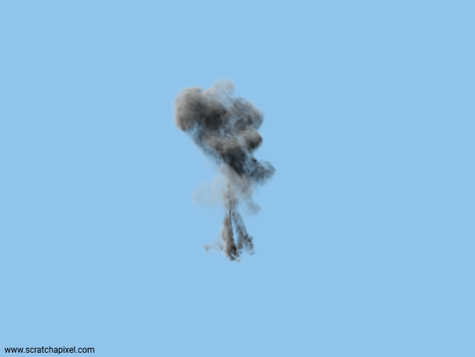
As you know, we aim to provide examples that have no dependency on external libraries. Consequently, we are not using an industry format such as OpenVDB (or Field3D, OpenVDB's ancestor) to store our grid data. Instead, we dumped the data of our fluid sim to a binary file in the most basic way using something similar to:
// our binary cache format
for (size_t z = 0; z < grid.res; ++z) {
    for (size_t y = 0; y < grid.res; ++y) {
        for (size_t x = 0; x < grid.res; ++x) {
            float density = grid.density[x][y][z];
            cacheFile.write((char*)&density, sizeof(float));
        }
    }
}
Note that OpenVDB works on the same principles, however, they support compression and things such as multi-resolution and sparse volumes (something we will touch on at the end of this lesson). Our approach has the merit of being straightforward which is what we look for when it comes to teaching and learning. So, what you need to pay attention to in the code above, is that we store slices of voxels back to front, along the z-axis. Keep in mind that (for a right-hand coordinate system) the minimum extent of our grid is located at the back of the grid, in the lower-left corner (the magenta voxel in the figure below). In voxel space, the first voxel in the grid has coordinates (0,0,0) and in our example, the last voxel (front of the grid, along the positive z-axis, in the upper-right corner) has coordinates (8,8,8) (the yellow voxel in the figure below. In this example, the grid resolution is 8).
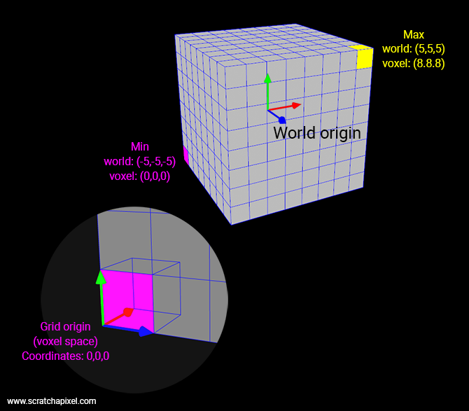
So if we map out the voxels in a simple float array like we do when we dumped the data out to the file (and when we read them back into memory from the file), the first voxel in this array as index 0 and the last voxel has index 511 (it's a 0-based array, so 8*8*8 minus 1). To compute the index of a voxel from its voxel-space coordinates, all we need to do is:
size_t index = (zi * gridResolution + yi) * gridResolution + xi;
This is the most basic way of getting a result. However, we can improve the image quality using what we call trilinear interpolation. Let's see how this works.
# Step 4: Improve the Result With a Trilinear Interpolation
The underlying idea is as follows: a voxel represents a single density value however a sample point can be located anywhere within the volume of any given voxel. Therefore it makes sense to assume that the density value at this location should somehow be a mix between the density of the voxel that the sample point is in as well as the density values of the voxels that are directly next to it as shown in the image below.

For the trilinear interpolation, we simply mix the values of 8 voxels. How do we mix them? Simply by calculating the distance from the sample point to each one of these 8 voxels and using these distances to weigh the contribution of each one of these 8 voxels to the final result.
The process is a linear interpolation but in 3D. The equation we are using to interpolate 2 values is \(a * (1 - weight) + b * weight\) where the \(weight\) varies from 0 and 1\. In 2D, this process is called a bilinear interpolation and requires 4 pixels. In 3D, we call this a trilinear interpolation and it requires 8 voxels. Note that the equation used to interpolate between a and b is called an interpolant. In the case of linear interpolation, the interpolant is a first-order polynomial.
We assume that the density stored in a given voxel is the value that the sample point should take if it was exactly in the middle of that voxel. Due to the nature of the trilinear interpolation scheme, to get that result, we need to shift the sample position in voxel space by -0.5\. Let's look at the code first and then explain how it works.
float evalDensity(const Grid* grid, const Point& p)
{
    Vector gridSize = grid.bounds[1] - grid.bounds[0];
    Vector pLocal = (p - grid.bounds[0]) / gridSize;
    Vector pVoxel = pLocal * grid.baseResolution;
    <span style="color: red; font-weight: 700;">Vector pLattice(pVoxel.x - 0.5, pVoxel.y - 0.5, pVoxel.z - 0.5);</span>
    int xi = static_cast<int>(std::floor(pLattice.x));
    int yi = static_cast<int>(std::floor(pLattice.y));
    int zi = static_cast<int>(std::floor(pLattice.z));

    float weight[3];
    float value = 0;

    // trilinear interpolation
    for (int i = 0; i < 2; ++i) {
        weight[0] = 1 - std::abs(pLattice.x - (xi + i));
        for (int j = 0; j < 2; ++j) {
            weight[1] = 1 - std::abs(pLattice.y - (yi + j));
            for (int k = 0; k < 2; ++k) {
                weight[2] = 1 - std::abs(pLattice.z - (zi + k));
                value += weight[0] * weight[1] * weight[2] * grid(xi + i, yi + j, zi + k);
            }
        }
    }

    return value;
}
Now let's see how (and why) this works.
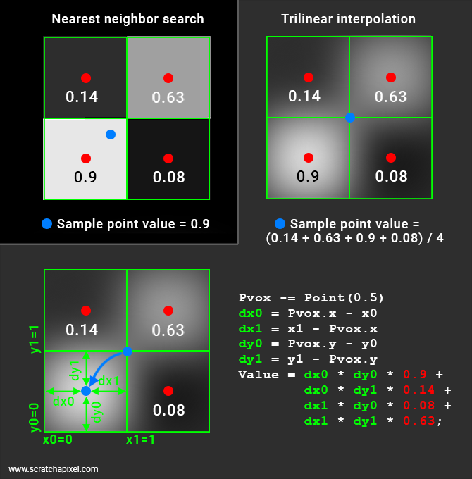
In the image above, the two techniques are illustrated. In the top-left corner, you have an example of the nearest-neighbor interpolation method. Nothing fancy here. We have 4 voxels (in the 2D case, 8 in 3D), and the sample point (the blue dot) falls in one of them. Therefore the sample point takes on the density value stored in that voxel.
Things get a little bit more complicated with the trilinear interpolation. You will probably agree that if our sample point was right in the middle of our four voxels, we should probably return the average of the density value stored in these four voxels. That is, in this particular example the sum of the voxel density values is divided by 4.
result = (0.9 + 0.14 + 0.08 + 0.63) / 4
Now this works ok if the point is right at the cross-over of four voxels which is an exceptional case. So we need to find a generic solution.
First (we will explain why we need to do this later), we need to offset our sample point by half a voxel space: (-0.5, -0.5, -0.5). If we keep the example of our sample point that falls exactly right in the middle of our four voxels, the sample point with the offset applied is now located right in the middle of the lower-left voxel. What we do next compute the distances from this point to each one of the voxel boundaries. In our illustration (2D case) this is represented by the distance dx0 (the distance from the sample point x coordinate to x0, the voxel lower-left x coordinate), dy0 (the distance from the sample point y coordinate to y0, the voxel lower-left y-coordinate), dx1 (the distance from the sample point x coordinate to x1, the voxel upper-right x-coordinate) and dy1 (the distance from the sample point y coordinate to y1, the voxel upper right y-coordinate). These are technically called the Manhattan distances.
Manhattan distance: the distance between two points measured along axes at right angles. In a plane with p1 at (x1, y1) and p2 at (x2, y2), it is |x1 - x2| + |y1 - y2|.
In practice, as we will see, we only need dx0, dy0, and dz0\. Here is the general idea of the trilinear interpolation again (check the lesson devoted to interpolation if you want a more complete explanation).
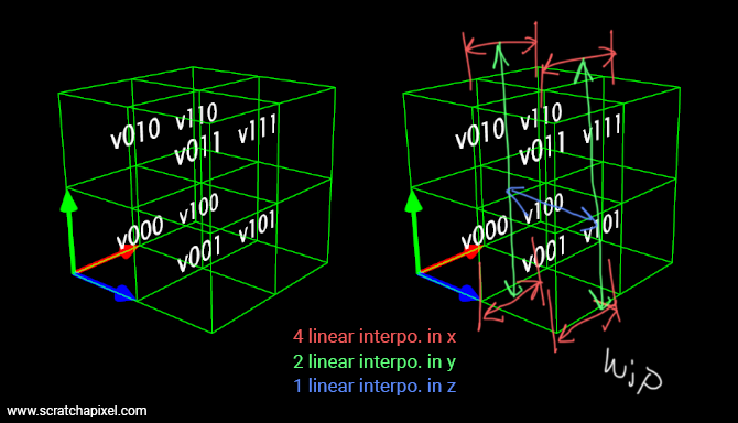
We have a block of 2x2x2 voxels. Let's call them v000, v100 (moving 1 voxel to the right), v010 (moving 1 voxel up), v110 (1 to the right, 1 up), v001 (moving 1 voxel forward), v101 (you get the idea by now), v011 and v111. The idea is to linearly interpolate v000-v100, v010-v110, v001-v1001, and v011-v111 using x0 as the weight. This gives us 4 values that we then linearly interpolate (in pairs again) using y0 as the weight. We are left with 2 values that we then finally linearly interpolate using z0 as the weight. Note that whether you start the first 4 linear interpolations with x0, y0 or z0 doesn't make any difference as long as you linearly interpolate the successive results using a different dimension each time. Remember that our linear interpolant is \(a * (1 - w) + b * w\) where \(w\) is the weight. In code, we get something like this:
float result =
    (1 - z0) * (  // blue
                (1 - y0) * (v000 * (1 - x0) + v100 * x0) + // green and red
                     y0  * (v010 * (1 - x0) + v110 * x0)   // green and red
                ) +
          z0 * ( // blue
                (1 - y0) * (v001 * (1 - x0) + v101 * x0) + // green and red
                     y0  * (v011 * (1 - x0) + v111 * x0)); // green and red
Hopefully, the layout helps you see the three nested levels of interpolation. With 4 (red) + 2 (green) + 1 (blue) interpolations. Now if we replace (1-x0), (1-y0), (1-z0), x0, y0, and z0 with wx0, wy0, wz0, wx1, wy1, and wz1 respectively, expand and rearrange the terms from the previous code snippet (2), we get:
float result =
    v000 * wx0 * wy0 * wz0 +
    v100 * wx1 * wy0 * wz0 +
    v010 * wx0 * wy1 * wz0 +
    v110 * wx1 * wy1 * wz0 +
    v001 * wx0 * wy0 * wz1 +
    v101 * wx1 * wy0 * wz1 +
    v011 * wx0 * wy1 * wz1 +
    v111 * wx1 * wy1 * wz1;
That's the code from our snippet 1 (though in snippet 1 the weights are calculated on the fly in nested loops). If you do the math using the 2D example from the image above where dx0 = dy0 = 0.5, we get:
result =
    0.9 * (1-dx0) * (1-dy0) + 0.14 * dx0 * (1-dy0) *  + 0.08 * (1-dx0) * dy0 + 0.63 * dx0 * dy0 =
    0.9 * 0.25 + 0.14 * 0.25 + 0.08 * 0.25 + 0.63 * 0.25
Which is the result we were looking for. Great, trilinear interpolation (bilinear in the 2D case) works. You also now understand why we need to offset the sample point by -0.5 in voxel space. This is required for the math to work. To be convinced, consider what happens when the sample point is right in the middle of the voxel (before we apply the offset). Once the offset is applied, the point will then lie right in the lower-left corner of the voxel (in 2D). That means that dx0 = dy0 (=dz0) =0 while all the other distances will be 1. And you get:
float result = grid.density(voxelX, voxelY, voxelZ) * (1-0) * (1-0) * (1-0) +
               0 + // 0 * (1-0) * (1-0)
               0 + // (1-0) * 0 * (1-0)
               0 + // 0 * 0 * (1-0)
               0 + // (1-0) * (1-0) * 0
               0 + // 0 * (1-0) * 0
               0 + // (1-0) * 0 * 0
               0;  // 0 * 0 * 0
In other words, the value returned for that sample will be the value stored in that voxel (0.9 in our example if we assume the sample point before the offset is in the middle of the lower-left voxel) which is exactly what you would expect.
That's all there is to a trilinear interpolation. Now let's see how different the result is compared to the nearest-neighbor method.
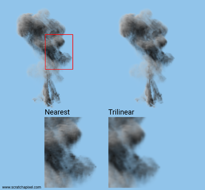
As you can see the image of the cache that was rendered using trilinear interpolation (right) is softer. Though this improvement comes at a price, as render time increases significantly when this method is used (compared to the nearest-neighbor method). A trilinear interpolation takes about 5 times as much as it takes to do a nearest-neighbor lookup (assuming no optimization).
Now you can read other people's code (again): OpenVDB
Let's see how OpenVDB does its trilinear interpolation:
template<class ValueT, class TreeT, size_t N>
inline bool
BoxSampler::probeValues(ValueT (&data)[N][N][N], const TreeT& inTree, Coord ijk)
{
    bool hasActiveValues = false;
    hasActiveValues |= inTree.probeValue(ijk, data[0][0][0]);  //i, j, k

    ijk[2] += 1;
    hasActiveValues |= inTree.probeValue(ijk, data[0][0][1]);  //i, j, k + 1

    ijk[1] += 1;
    hasActiveValues |= inTree.probeValue(ijk, data[0][1][1]);  //i, j+1, k + 1

    ijk[2] -= 1;
    hasActiveValues |= inTree.probeValue(ijk, data[0][1][0]);  //i, j+1, k

    ijk[0] += 1;
    ijk[1] -= 1;
    hasActiveValues |= inTree.probeValue(ijk, data[1][0][0]);  //i+1, j, k

    ijk[2] += 1;
    hasActiveValues |= inTree.probeValue(ijk, data[1][0][1]);  //i+1, j, k + 1

    ijk[1] += 1;
    hasActiveValues |= inTree.probeValue(ijk, data[1][1][1]);  //i+1, j+1, k + 1

    ijk[2] -= 1;
    hasActiveValues |= inTree.probeValue(ijk, data[1][1][0]);  //i+1, j+1, k

    return hasActiveValues;
}

template<class ValueT, size_t N>
inline ValueT
BoxSampler::trilinearInterpolation(ValueT (&data)[N][N][N], const Vec3R& uvw)
{
    auto _interpolate = [](const ValueT& a, const ValueT& b, double weight)
    {
        const auto temp = (b - a) * weight;
        return static_cast<ValueT>(a + ValueT(temp));
    };

    // Trilinear interpolation:
    // The eight surrounding lattice values are used to construct the result. \n
    // result(x,y,z) =
    //     v000 (1-x)(1-y)(1-z) + v001 (1-x)(1-y)z + v010 (1-x)y(1-z) + v011 (1-x)yz
    //   + v100 x(1-y)(1-z)     + v101 x(1-y)z     + v110 xy(1-z)     + v111 xyz

    return  _interpolate(
                _interpolate(
                    _interpolate(data[0][0][0], data[0][0][1], uvw[2]),
                    _interpolate(data[0][1][0], data[0][1][1], uvw[2]),
                    uvw[1]),
                _interpolate(
                    _interpolate(data[1][0][0], data[1][0][1], uvw[2]),
                    _interpolate(data[1][1][0], data[1][1][1], uvw[2]),
                    uvw[1]),
                uvw[0]);
}

template<class TreeT>
inline bool
BoxSampler::sample(const TreeT& inTree, const Vec3R& inCoord,
                   typename TreeT::ValueType& result)
{
    ...
    const Vec3i inIdx = local_util::floorVec3(inCoord);
    const Vec3R uvw = inCoord - inIdx;

    // Retrieve the values of the eight voxels surrounding the
    // fractional source coordinates.
    ValueT data[2][2][2];

    const bool hasActiveValues = BoxSampler::probeValues(data, inTree, Coord(inIdx));

    result = BoxSampler::trilinearInterpolation(data, uvw);

    ...
}
The sample() method is first fetching the values stored in the 8 voxels. This happens in the method probeValues. Then, the voxels are interpolated as described above (in the trilinearInterpolation method). The function _interpolate is nothing else than a linear interpolation more often called lerp in code.
Going further with volume caches
We are just listing a series of topics that we think are worth mentioning here for reference. To keep this lesson reasonably short, we won't get into much detail for now. Most of these topics will be either developed in a future revision of this lesson or studied in separate lessons.
Other interpolation schemes: cubic and filter kernels
As mentioned earlier, the linear interpolant is a first-order polynomial. It is possible to use higher-order polynomials for smoother results. You can for example use cubic interpolation. In 2D, we need to sample 4x4 pixels to perform a bicubic interpolation. In 3D, we need \(2^4=64\) voxels. As you can imagine, the result will look smoother, but the render time will increase.
You can also use filter kernels, similar to those used in image filtering (such as a triangle, Mitchell, or Gaussian filter kernels). Like with images, the larger the filter's extent, the longer the processing time.
Both techniques will be fully explained in a future revision of this lesson.
Storing more data alongside density
Volume cache formats used in production are generally designed to let you store any channel you want in the cache alongside the density such as the temperature (useful to render fire), the velocity (useful to render 3D motion blur), etc.
Filtering and brick maps
If you render volume caches for production purposes, you should probably care about filtering and LODs. The problem you may have with rendering volume caches is the same as with rendering textures. Textures have a fixed resolution (number of pixels like 512, 1024, and so on) and if you render an object to which a given texture is applied from super far away, then you assume your object is just a few pixels wide in the image, as the object moves or the camera moves, each time a new frame is rendered different pixels or texels from the textures will be rendered. As a result, the texture will appear to jiggle (to say the least, but it more often simply looks like a kind of noise) from frame to frame. To minimize this problem, we make smaller versions of the texture stored alongside the original texture data; we call these lower-resolution versions of the original texture mipmaps. Using a lower resolution of the texture when the object is far away (small in the image) removes the noise (technically called aliasing). We haven't touched on the topic of mipmap yet, but we will soon.
In the meantime and if you are already familiar with the concept of mipmap, what they are, what they are used for, and how to create them, you should know that the problem we have with filtering 2D textures is also a problem we have with 3D caches (or 3D textures for that matter). Therefore, we can adapt the mipmap method to 3D caches. For that, you need to create downsized versions of the original grid data and use the right level (downsized version), based on how small the cache is in the image. While the process is very similar to mipmaps and while you can call these downsized versions mipmaps as well, in 3D we call them brick maps instead. They look like Minecraft objects.
The term brick map was coined by the Pixar Renderman's team we believe it but we are not too sure about its origin... if someone knows, please write to us about it. But generally, the idea of having a cache storing multiple resolutions of its data is not particularly new or uncommon. It's probably supported by all production renderers and formats such as OpenVDB.
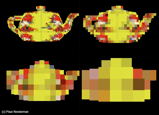
Building these brick maps is very similar to building the texture's mipmap levels, however, we are taking the average of 8 voxels (instead of taking the average of 4 pixels or texels). That's why dealing with grids whose resolution is exactly a power of 2 is convenient, as downsizing the levels becomes trivial in this case.
Here is some code that shows how you can create these levels from our original fluid sim caches (their base resolution at level 0 is 128). This is just a quick example for now until we get a chance to address this topic properly:
size_t baseResolution = 128;
size_t numLevels = log2(baseResolution); /* float to size_t implicit cast */
std::unique_ptr<Grid []> gridLod = std::make_unique<Grid []>(numLevels - 2); // ignore res. 2 and 4

// load level 0 data
gridLod[0].baseResolution = baseResolution;
std::ifstream ifs;
char filename[256];
sprintf_s(filename, "./grid.%d.bin", frame);
ifs.open(filename, std::ios::binary);
gridLod[0].densityData = std::make_unique<float[]>(baseResolution * baseResolution * baseResolution);
ifs.read((char*)gridLod[0].densityData.get(), sizeof(float) * baseResolution * baseResolution * baseResolution);
ifs.close();

for (size_t n = 1; n < numLevels - 2; ++n) {
    baseResolution /= 2;
    gridLod[n].baseResolution = baseResolution;
    gridLod[n].densityData = std::make_unique<float[]>(baseResolution * baseResolution * baseResolution);
    for (size_t x = 0; x < baseResolution; ++x) {
        for (size_t y = 0; y < baseResolution; ++y) {
            for (size_t z = 0; z < baseResolution; ++z) {
                gridLod[n](x, y, z) =
                    0.125 * (gridLod[n - 1](x * 2,     y * 2,     z * 2) +
                             gridLod[n - 1](x * 2 + 1, y * 2,     z * 2) +
                             gridLod[n - 1](x * 2,     y * 2 + 1, z * 2) +
                             gridLod[n - 1](x * 2 + 1, y * 2 + 1, z * 2) +
                             gridLod[n - 1](x * 2,     y * 2,     z * 2 + 1) +
                             gridLod[n - 1](x * 2 + 1, y * 2,     z * 2 + 1) +
                             gridLod[n - 1](x * 2,     y * 2 + 1, z * 2 + 1) +
                             gridLod[n - 1](x * 2 + 1, y * 2 + 1, z * 2 + 1));
			}
		}
	}
}
...
// to render level 3 of the cache for example (resolution: 16)
trace(ray, L, transmittance, rc, gridLod[3]);
...
We won't explain how to select the right level for now, but we will in a future revision of the lesson. In the meantime, at least you are aware of the problem and what the solution could be.
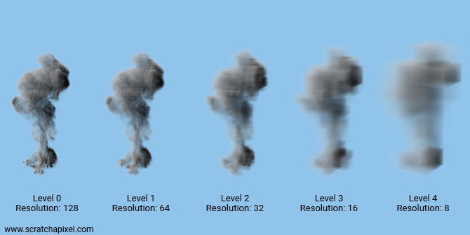
Here is an image of our cache rendered at different levels (level 0 is the original cache resolution, that is 128 in our example):
Motion blur
What about 3D motion blur? To render this effect we need to store the voxel with the motion of the fluid. This is typically represented as a direction called the motion vector. This vector's direction indicates in which average direction the fluid is moving through the grid; its magnitude is how fast the fluid moves. Using this information, 3D motion blur can be simulated at render time.
This topic will be studied in a future lesson.
Advection
While advection is not directly related to volume rendering (it has more to do with fluid simulation), we are adding it here as a reminder (so that we can write a lesson about it in the future if we can). It can be done at render time to add details to an existing fluid sim.
Sparse volumes: what are they?
A lot of the time, only a fraction of the voxels in a grid are storing density values that are greater than 0. That leaves a lot of "empty" voxels; storing them can potentially be a significant waste. Similarly, you may have a group of 8 voxels storing the same density value for example 0.138. This is also a waste of space. Sparse volumes were designed to address this issue.
The general idea is like this: we create a voxel that has the size of a block of 2x2x2 voxels. Therefore this bigger voxel is twice the size of the original voxels. Next: if all the voxels in the block of 2x2x2 voxels have the same density value (it can be 0 or any value greater than 0 for example 0.139), we then delete the group of 2x2x2 voxels and store the single value in the larger voxel (say 0.139 to follow our example), otherwise, the bigger voxel points to the original block of 2x2x2 voxels.
This process is recursive. We start from the highest resolution grid (highest level), then build the lower levels from the bottom up. Voxels pointing to blocks of more voxels are internal nodes whereas voxels storing a value are leaf nodes. The image below shows an example of a sparse 2D volume.
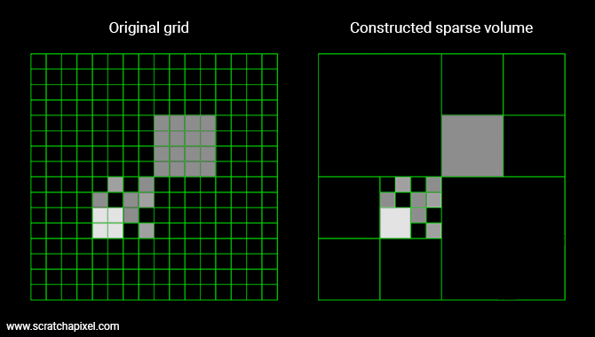
When a block isn't merged, we store 1 (the bigger voxel) + 8 voxels (the block of 2x2x2 voxels), but when a block is merged, we only store 1 voxel. In most fluid simulations, a large percentage of the original voxels are either empty or share similar density values. This for example is often the case with clouds. The core of a cloud is generally quite homogeneous. Density varies essentially at the edge of the cloud. So encoding these volumes with a sparse representation can be a great way of reducing the size of the cache on disk and in memory.
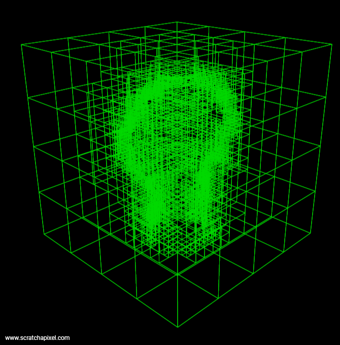
Note that using blocks of 2x2x2 voxels is not mandatory. Many systems including OpenVDB, choose an octree structure for the first few upper levels of the hierarchy but then store the following levels into blocks of 32x32x32 voxels (for example). Organizing data that way might improve cache coherency and data access (compared to using smaller block sizes).
Finally, sparse volumes are also useful in rendering. Large voxels that are empty can be skipped. Large voxels with uniform density can be rendered as homogenous volumes. Added together, these allow for potentially large time savings.
The topic of sparse volumes (that share similarity with LODs and brick maps) is important and large enough to deserve a lesson of its own. In the meantime, if you are interested in the topic, you can also search for Gigavoxels (an octree of bricks).
Out-of-core rendering
There's a reason why we mention out-of-core rendering right after sparse volume. Sparse volumes and octrees of bricks have often been designed (besides the optimizations we mentioned above) to make it possible to render very large volume caches, that wouldn't normally be renderable as a grid, due to memory limitations.
When you can't load the entire file in memory (you don't want to be limited in how large your simulation might be), what you do is only load from the cache (using a kind of buffer mechanism), the bricks that you need (those for example that are visible to the camera). This is of course only possible if your volume cache is organized as a collection of bricks that can be loaded on the fly (on demand). This topic will be covered in full in a future lesson.
Mind how you iterate through the grid data
If you need to iterate through the voxels, it's best to do it that way:
for (size_t x = 0; x < resolution; ++x) {
    for (size_t y = 0; y < resolution; ++y) {
        for (size_t z = 0; z < resolution; ++z) {
            ...
        }
    }
}
Rather than that way:
for (size_t z = 0; z < resolution; ++z) {
    for (size_t y = 0; y < resolution; ++y) {
        for (size_t x = 0; x < resolution; ++x) {
            ...
        }
    }
}
This is because of the way data is laid out in memory. By iterating over x first and z last, we are iterating through the values stored in memory sequentially. By iterating over z first and x last, we would be jumping to different parts of the memory. This is likely to generate a lot of cache misses which decreases performance. Of course, this depends on the format. We stored the data in the cache by iterating through x first, then y, then z but other formats might be using a different convention. So be mindful of this particular aspect of your code, as this might be a place to look for optimizations.
Baking the lighting
You can bake the lighting in the grid's voxels and read this data from the voxels at render time to skip the step of evaluating the Li term at each raymarching step on the camera ray. This will speed up your rendering. Of course, you will still need to render this Li term for each voxel in the grid in pre-pass (the baking pass) which is still going to take a while. Furthermore, you will need to start baking again whenever the lighting or the simulation changes. We are mostly mentioning this technique for reference and historical reasons.
Deep shadow maps
Shadow maps are about to become an artifact of the past, though again for the sake of completeness and historical reasons, we thought it would be great to mention deep shadow maps, which in a way have similarities with the idea of baking the lighting into the grid's voxels. The idea here is to compute a shadow map per light in the scene. But rather than storing the depth from the light to the nearest object in the scene for any given pixel (which is what shadow maps are used for), deep shadow maps store the density of the volume instead as a function of distance. In other words, each pixel in the deep shadow maps stores a curve that represents how transmission through the volume changes as we move through it. This technique was developed in 2000 by Tom Lokovic and Eric Veach from Pixar (you can find their paper here if you want to learn more about it). Several variations of that technique exist.
Source Code
As usual, you can find the source code for this chapter in the source code section of this lesson. We also provide a sequence of about 100 cache files (download the cachefiles.zip file and unzip it on your local drive alongside the program source code) which you can use to render the animation shown at the beginning of this chapter.