Volume Rendering

The Ray-Marching Algorithm

The almighty ray-marching algorithm

To integrate incoming light along the ray due to in-scattering, we will break down the volume that the ray passes through into small volume elements and combine the contribution of each of these small volume elements to the overall volume object, a little bit like when we stack images with a mask or alpha channel (generally representing the objects' opacity) onto each other in a 2D editing software (such as Photoshop). That is why we spoke about the alpha compositing method in the first chapter. Each one of these small volume elements represents a sample in the Riemann sum mentioned in the first chapter.

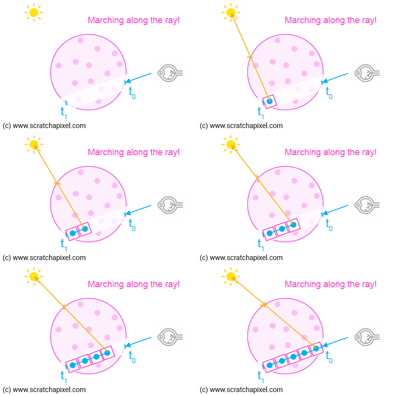
The algorithm works as follows:

1. Find the value for t0 and t1, the points where the camera/eye ray enters and leaves the volume object.

2. Divide the segment defined by t0-t1 into X number of smaller segments of identical size. Generally, we do so by choosing what we call a step size, which is nothing else than a floating number defining the length of the smaller segment. So for instance, if t0=2.5, t1=8.3, and the step size = 0.25, we will divide the segment defined by t0-t1 by (8.3-2.5)/0.25=23 smaller segments (let's keep it simple for now, so don't worry about the decimals).

3. What you do next is "march" along the camera ray X times, starting from either t0 or t1 (see bullet point #6).

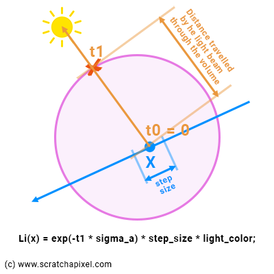
5. Each time we take a step, we shoot a "light ray" starting from the middle of the step (our sample point) to the light. We compute where the light ray intersects (leaves) the volume element, and compute its contribution to the sample (due to in-scattering) using Beer's Law. Remember, light coming from the light source is absorbed by the volume as it travels through it to the sample point. This is the Li(x) value in the Riemann sum that we mentioned in the previous chapter. Don't forget that we need to multiply this value by step size which in the Riemann sum, corresponds to the dx term, the width of our rectangle. In pseudo-code we get:

// compute Li(x) for current sample x
float lgt_t0, lgt_t1; // parametric distance to the points where the light ray intersects the sphere
volumeSphere->intersect(x, lgt_dir, t0, lgt_t1); // compute the intersection of the light ray with the sphere
color Li_x = exp(-lgt_t1 * sigma_a) * light_color * step_size; // step_size is our dx
...

As you can see in Figure 2, t0 for the light ray-sphere intersection test should always be 0 because the light ray starts from within the sphere, and t1 is the parametric distance to the point where the light ray intersects the sphere from our sample position x. So we can use that value in Beer's law equation for the distance over which light is absorbed by the volumetric object.

6. Then of course light passing through the small volume element (our sample) is attenuated as it passes through the sample as well. So we compute the transmission value for our sample using the step size as the value for the distance traveled by the light beam through the volume in Beer's law equation. And then attenuate (multiply) the light amount (in-scattering) by this transmission value.

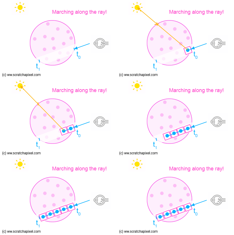
7. Finally we need to combine each one of the samples to account for their respective contribution to both the overall opacity and "color" of the volumetric object. Indeed, if you think of this process backward (like shown in Figure 1), the first volume element (starting from t1) is occluded by the second, which is itself occluded by the third one, etc. until we reach the last element in the "queue" (the sample that's directly next to t0). If you look "through the camera" ray, the element directly next to t1 is occluded by all the elements that are in front of it. The sample that's just after the sample that's directly next to t0 is occluded by that very first sample, etc.

We can combine samples in two ways: either backward (marching from t1 to t0) or forward (marching from t0 to t1). One is better than the other (sort of). We will now describe how they work.

Backward Ray-Marching.

In backward ray-marching, we will march along the ray from back to front. In other words from t1 to t0. This changes the way we combine the samples to compute the final pixel opacity and color values.

Quite naturally, since we start from the back of the volumetric object (our sphere), we could initialize our pixel color (the color returned for that camera ray) with the background color (our bluish color). But in our implementation, we will only combine the two at end of the process (once we have computed the volumetric object color and opacity), a little bit like when we compose two images in a 2D editing software.

We will compute the contribution of our first sample (say X0) in the volume, starting as we mentioned from t1, and walk back to t0, taking regular steps (defined by step size).

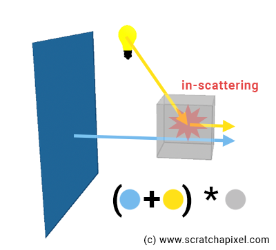
What is the contribution of that sample?

• We will compute the in-scattering contribution (the contribution of the light source) Li(X0) as explained above (point #6): shooting a light ray in the direction of the light, then attenuate the light contribution using Beer's law to account for how much of the light is absorbed by the volumetric object as it traveled from the point where it entered the object (our volume sphere) to our sample point (X0).

• Then, we need to multiply that light by the sample's transparency value (which represents how much of that light is being absorbed by the sample). The sample transparency is computed using Beer's law again, using step size as the distance traveled by the light beam through that sample (figure 3).

...
color Li_x0 = exp(-lgt_t1 * sigma_a) * light_color * step_size; // step_size is our dx
color x0_contrib = Li_x0 * exp(-step_size * sigma_a);
...

We've just computed our first sample X0. We then move to our second sample (X1), but now we have two sources of light that we need to account for: the light beam coming from the first sample X0 (our previous result), and the light beam passing through the second sample due to in-scattering, X1\. We already computed the former (as we just said, that's our previous result) and we know how to render the latter. We sum them up and multiply this sum by the second sample transmission value. This becomes our new result. And we keep repeating this process with X2, X3, ... until we eventually reach t0\. The final result is the contribution of the volumetric object to the current camera ray pixel's color. This process is illustrated below.

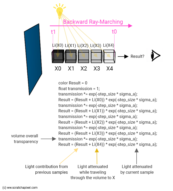
Note from the image above that we compute two values: the volume overall color (stored in the result) and the overall volume transparency. We initialize this value to 1 (fully transparent) and then attenuate the value with each one of the sample transparency values as we walk up (or down) the ray (from t1 to t0). We can then (finally) use this overall transparency value to combine the volume object over our background color. We simply do:

color final = background_color * transmission + result;

In compositing terms, we would say that the "result" term is already pre-multiplied by the volume overall transparency. But if this is confusing to you, we will clarify this point in the next chapter. So don't focus on this too much for now.

Note also that both in the image above and in the code below the attenuation term of the samples is always the same: exp(-step_size * sigma_a). Of course, this is not efficient. You should compute this term once, store it in a variable, and use that variable instead. But clarity is our goal, not writing performant code. Besides, for now, this value is constant as we march along the ray but we will discover in the next chapters that it will eventually vary from sample to sample.

This is what it looks like translated into code:

constexpr vec3 background_color{ 0.572f, 0.772f, 0.921f };

vec3 integrate(const vec3& ray_orig, const vec3& ray_dir, ...)
{
    const Object* hit_object = nullptr;
    IsectData isect;
    for (const auto& object : objects) {
        IsectData isect_object;
        if (object->intersect(ray_orig, ray_dir, isectObject)) {
            hit_object = object.get();
            isect = isect_object;
        }
    }

    if (!hit_object) 
        return background_color;

    float step_size = 0.2;
    float sigma_a = 0.1; // absorption coefficient
    int ns = std::ceil((isect.t1 - isect.t0) / step_size);
    step_size = (isect.t1 - isect.t0) / ns;

    vec3 light_dir{ 0, 1, 0 };
    vec3 light_color{ 1.3, 0.3, 0.9 };

    float transparency = 1; // initialize transparency to 1
    vec3 result{ 0 }; // initialize the volume color to 0

    for (int n = 0; n < ns; ++n) {
        float t = isect.t1 - step_size * (n + 0.5);
        vec3 sample_pos= ray_orig + t * ray_dir; // sample position (middle of the step)

        // compute sample transparency using Beer's law
        float sample_transparency = exp(-step_size * sigma_a);
        
        // attenuate global transparency by sample transparency
        transparency *= sample_transparency;

        // In-scattering. Find the distance traveled by light through 
        // the volume to our sample point. Then apply Beer's law.
        IsectData isect_vol;
        if (hitObject->intersect(sample_pos, light_dir, isect_vol) && isect_vol.inside) {
            float light_attenuation = exp(-isect_vol.t1 * sigma_a);
            result += light_color * light_attenuation * step_size;
        }

        // finally attenuate the result by sample transparency
        result *= sample_transparency;
    }

    // combine with background color and return
    return background_color* transparency + result;
}

But mindful of this code. It's not accurate yet. It's missing a few terms that we will be looking at in the next chapter. For now, we just want you to understand the principle of ray-marching. Yet this code will produce a convincing image.

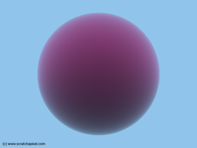
Note that in this example, we've been using a top-down distant light (light direction is upward along the y-axis). The reddish color of the sphere comes from the light color. You can see that the top half of the sphere is brighter than the bottom half. The shadowing effect is visible already.

Let's see again what happens to the samples as we march along the ray:

If you look at what happens to just \(Li(X_0)\) as we go through the loop, you can observe that it gets multiplied by the sample attenuation raised to some power. The more we march along the ray, the higher the exponent (first 1, then 2, then 3, ...) and thus the smaller the result (since the attenuation or sample transparency is lower than 1). In other words, the contribution of the first sample to the overall resulting light scattered by the volume decreases as more samples are accumulated.

Forward Ray-Marching.

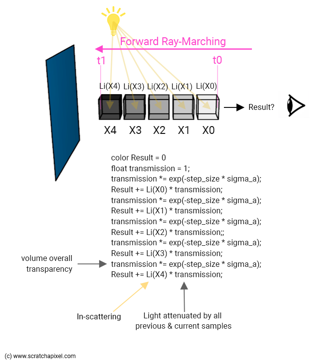
There is no difference with backward ray-marching when it comes to computing Li(x) and the sample's transmission value. What is different is how we combine samples because this time around, we will march from t0 to t1 (from front to back). In forward ray-marching, the contribution of light scattered by a sample has to be attenuated by the overall transmission (transparency) value of all samples (including the current one) that we've been processing so far: Li(X1) is attenuated by the transmission values of the samples X0 and X1, Li(X2) is occluded by the transmission values of the samples X0, X1, and X2, etc. Here is a description of the algorithm:

• Step 1: before we enter the ray-marching loop: initialize the overall transmission (transparency) value to 1 and the result color variable to 0 (the variable that stores the volumetric object color for the current camera ray): float transmission = 1; color result = 0;.

• Step 2: for each iteration in the ray-marching loop:

  • Compute in-scattering for the current sample: Li(x).

  • Update the overall transmission (transparency) value by multiplying it by the current sample transmission value: transmission *= sample_transmission.

  • Multiply Li(x) by the overall transmission (transparency) value: light scattered by the sample is occluded by all samples (including the current sample) that we've been processing so far. Add the result to our global variable that stores the volume color for the current camera ray: result += Li(x) * transmission.

Translated into code:

...
vec3 integrate(const vec3& ray_orig, const vec3& ray_dir, ...)
{
    ...
    float transparency = 1; // initialize transparency to 1
    vec3 result{ 0 }; // initialize the volume color to 0

    for (int n = 0; n < ns; ++n) {
        float t = isect.t0 + step_size * (n + 0.5);
        vec3 sample_pos = ray_orig + t * ray_dir;

        // current sample transparency
        float sample_attenuation = exp(-step_size * sigma_a);

        // attenuate volume object transparency by current sample transmission value
        transparency *= sample_attenuation;

        // In-Scattering. Find the distance traveled by light through 
        // the volume to our sample point. Then apply Beer's law.
        if (hit_object->intersect(sample_pos, light_dir, isect_vol) && isect_vol.inside) {
            float light_attenuation = exp(-isect_vol.t1 * sigma_a);
            // attenuate in-scattering contrib. by the transmission of all samples accumulated so far
            result += transparency * light_color * light_attenuation * step_size;
        }
    }

    // combine background color and volumetric object color
    return background_color * transparency + result;
}

But mindful of this code. It's not accurate yet. It's missing a few terms that we will be looking at in the next chapter. For now, we just want you to understand the principle of ray-marching. Yet this code will produce a convincing image.

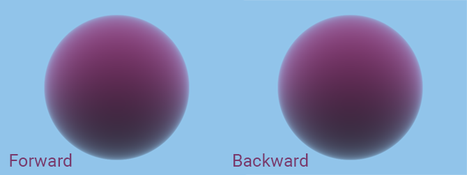
No need to show an image here. If we've done it right, backward and forward ray-marching should give the same result. Ok, we knew you wouldn't take this for granted, so here are the results.

Why is forward ray-marching "better" than backward ray-marching?

Because we can stop ray-marching as soon as the transparency of the volume gets very close to 0 (which would happen if the volume is large enough and/or the scattering coefficient is high enough). And this is possible only if you ray-march moving forward.

Right now, rendering our volume sphere is rather quick but you will see as we progress through the chapters that it will eventually get slow. So, if we can avoid computing samples that aren't contributing to the pixel's color because we reached a point as we march along the ray where we know that the volume is opaque, then it's a good optimization.

We will implement this idea in the next chapter.

Choosing the Step Size

Remember that the reason why we ray-marching, take small steps from t0 to t1 is to estimate an integral (the amount of light scattered towards the eye along the camera ray due to in-scattering) using the Riemann sum method. As explained in the chapter before and in the lesson the mathematics of shading, the larger the rectangles (the width of the rectangles in our case are defined by the step size here) used to estimate the integral the less accurate the approximation. Or the other way around: the smaller the rectangle (the smaller the step size) the more accurate the estimation, but of course the longer it takes to calculate. For now, rendering our volumetric sphere is rather fast, but as we progress through the lesson, you will see that it will eventually get much much slower. This is why choosing the step size is a tradeoff between speed and accuracy.

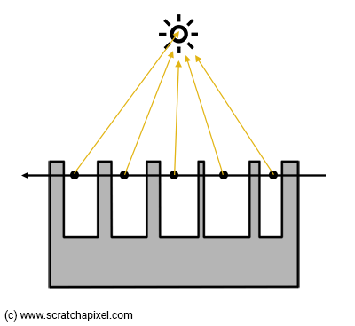
For now, we assume the volume density is also uniform. In the next chapters, we will see that to render volume density such as clouds or smoke, the density varies through space. Such volumes are made of large frequency features but also smaller ones. If the step size is too large it might eventually fail to capture some of these smaller frequency features (Figure 5). This is a filtering issue, an important but complex topic on its own.

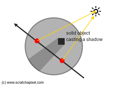
Another problem might arise that requires tweaking the step size: shadows. If small solid objects are casting shadows on the volumetric object, you will eventually miss them if the step size is too large (Figure 6).

All that doesn't tell us how to choose a good step size. In theory, there's no rule. You should essentially have an idea of the size of your volumetric object. For example, if it's a rectangle filling up a room with some kind of uniform atmosphere, you should get an idea of the size of that room (and of the kind of units you use, like 1 unit = 10 centimeters for example). So if the room is 100 units large, a step size of 0.1 might be too small whereas 1 or 2 might be a good place to start. Then you need to fiddle around to find a good tradeoff between speed and accuracy as we mentioned before.

Now, this is not entirely true either. While choosing the step size empirically by considering how big the objects are in the scene, there must be a more rational way of doing so. One possible way is to consider "how big" is the pixel at the distance where we enter the volume object and set the step size to the dimension of the projected pixel. Indeed, a pixel that is a discrete object can't represent details from the scene that are smaller than its size. We won't get into much more detail here because filtering is worth a lesson on its own. All we will say, for now, is that a good step size is close to the projected size of a pixel at the point where the camera ray intersects the volume. This can be estimated with something like:

float projPixWidth = 2 * tanf(M_PI / 180 * fov / (2 * imageWidth)) * tmin;

Which you can optimize if you wish to. Where tmin is the distance where the camera ray intersects the volume object. One could similarly compute the projected pixel width where the ray leaves the volume and linearly interpolate the projected pixel width at tmin and tmax to set the step size as we march along the ray.

Other considerations of interest before we move on!

Writing production code would require storing the ray opacity and color with the ray data. So that we can ray-trace the solid objects first, then the volumetric objects and combine the result as we go (in a similar fashion to what we did by combining the background color with the volumetric sphere object in the example above).

Note that several volumetric objects can be on the camera ray's path. Hence the necessity of storing the opacity along the way and combining the consecutive volumetric objects' opacity and color as we ray-march them.

A volumetric object can be made of a collection of combined objects such as cubes or spheres overlapping each other. In this case, we may want to combine them in some sort of aggregate structure. Ray-marching such aggregates require computing the intersection boundaries of the objects making the aggregate with special care.

Next: add the missing terms to get a physically accurate result.

In the third/next chapter of this lesson, we will add some of the terms that are missing to our current implementation to get a result that's physically (more) accurate. We will also show you that equipped with this knowledge, you should now be ready to read and understand other's people renderer's code. Ready?

Source Code

The source code to reproduce the images of the first two chapters is available for download with compilation instructions (embedded within the file) in the last chapter of the lesson (as usual). Be aware though the code is a bit different from the code snippets that were shown in this chapter. The differences are explained in the next chapter.