Volume Rendering

Ray Marching: Getting it Right!

Reading time: 28 mins.

In-Scattering and Out-Scattering.

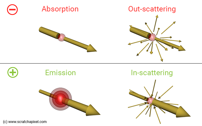
In the previous chapters, we only accounted for two types of interactions between light beams and particles making up the medium: absorption and in-scattering. But, to get an accurate result, we should consider four types. We can divide them into two categories. Interactions that attenuate the energy of light beams as they pass through the medium to the eye. And those that contribute to increasing their energy.

Light beams traveling to the eye through the medium lose energy due to:
- Absorption: a portion of the light energy is absorbed by the particles making up the medium. If you were the particle you could say: "some light is traveling to you, you the viewer, but sorry I decided to eat some of it, so you'll get less."
- Out-scattering: as mentioned in the previous chapter, light is scattered by particles. This causes light that's not traveling toward the eye, to somehow be redirected toward the eye. This is the in-scattering effect we have described in the previous chapter. But light that's traveling towards the eye can also be scattered out on its way to the eye. And that means that light loses energy due to this effect as well. This is called out-scattering (naturally). If you were the particle you could say: "some light is traveling to you, you the viewer, but I decided to scatter some of it into some random directions, so you'll get less."
Light beams traveling to the eye through the medium gain energy due to:
- Emission: we mentioned this effect in the first chapter but also mentioned we would ignore it for now. A flame for example can emit incandescent light.
- In-Scattering: we are already familiar with this effect. Some of the light that's not initially traveling toward the eye is being redirected toward the eye due to scattering. This effect is called in-scattering. If you were the particle you could think of this effect in this term: "I gathered light that's coming to me from all directions and spit out some of it in your direction, you the viewer, so you'll get some light that wasn't initially meant for you". You can see in-scattering as a result of out-scattering; light is scattered in all directions (more or less as we will see when we introduce the phase function later). It just happens that one of that directions is the viewing direction (the eye or camera ray).

These effects are illustrated in the image below.

In our computation for how much light we lose as light travels through the medium to the eye, we have to account for both absorption and out-scattering. Both out- and in-scattering are caused by the same type of light-particle interaction: scattering which, in the previous chapter, we've been defining with the variable $\sigma_s$ (the Greek letter sigma). So since scattering ($\sigma_s$) is also responsible for how much light we lose as light travels through the medium to the eye, we need to account for it in our Beer's law equation alongside the absorption coefficient $\sigma_a$. Remember, this equation is used to both compute the term Li(x) and the sample transmission value. Our code thus now becomes (changes in red):

...
float sigma_a = 0.5; // absorption coefficient
float sigma_s = 0.5; // scattering coefficient
// compute sample transmission
float sample_attenuation = exp(-step_size * (sigma_a + sigma_s)); 
transparency *= sample_attenuation; 
 
// In-scattering. Find the distance light travels through the volumetric sphere to the sample.
// Then use Beer's law to attenuate the light contribution due to in-scattering.
if (hit_object->intersect(sample_pos, light_dir, isect_vol) && isect_vol.inside) { 
    float light_attenuation = exp(-density * isect_vol.t1 * <span style="color: red; font-weight: bold; background-color: rgba(255,0,0,0.1);">(sigma_a + sigma_s)</span >); 
    result += ...; 
}
...

Sometimes you will see the terms $\sigma_a$ and $\sigma_s$ summed up in a term called the extinction coefficient often denoted $\sigma_t$ (sigma t).

$$\sigma_t = \sigma_a + \sigma_t$$

We are not entirely done with the scattering term... How much light is being scattered towards the eye due to in-scattering is also proportional to the scattering term. So we need to multiply the light contribution due to in-scattering by the $\sigma_s$ variable as well. Our code becomes (changes in red):

...
float sigma_a = 0.5; // absorption coefficient
float sigma_s = 0.5; // scattering coefficient
// compute sample transmission
float sample_attenuation = exp(-step_size * (sigma_a + sigma_s)); 
transparency *= sample_attenuation; 
 
// In-scattering. Find the distance light travels through the volumetric sphere to the sample.
// Then use Beer's law to attenuate the light contribution due to in-scattering.
if (hit_object->intersect(sample_pos, light_dir, isect_vol) && isect_vol.inside) { 
    float light_attenuation = exp(-isect_vol.t1 * (sigma_a + sigma_s)); 
    result += transparency * light_color * light_attenuation * <span style="color: red; font-weight: bold; background-color: rgba(255,0,0,0.1);">sigma_s</span> * step_size; 
}
...

The Density Term

We will speak about this term in detail in the next chapter.

Now so far we considered that the scattering and absorption coefficient which we have been using to control how "opaque" the volume is (remember that the higher these coefficients, the more opaque the volume) is uniform across the volume itself. In the scientific literature, this is often referred to as a homogenous participating medium. This is generally not the case with "volumes" in the real world. Think of clouds or smoke plumes for example. Their opacity varies spatially. We then speak of heterogeneous participating medium.

We will only see how to simulate volumetric objects with varying densities in the next chapter, but for now, let's just say that we want some kind of variables that will scale our scattering and absorption coefficient globally. Let's call this variable density. We will use it to scale both $\sigma_a$ and $\sigma_s$ as follows (changes in red):

...
float sigma_a = 0.5; // absorption coefficient
float sigma_s = 0.5; // scattering coefficient
<span style="color: red; font-weight: bold; background-color: rgba(255,0,0,0.1);">float density = 1;</span>
// compute sample transmission
float sample_attenuation = exp(-step_size * <span style="color: red; font-weight: bold; background-color: rgba(255,0,0,0.1);">density</span> * (sigma_a + sigma_s)); 
transparency *= sample_attenuation; 
 
// In-scattering. Find the distance light travels through the volumetric sphere to the sample.
// Then use Beer's law to attenuate the light contribution due to in-scattering.
if (hit_object->intersect(sample_pos, light_dir, isect_vol) && isect_vol.inside) { 
    float light_attenuation = exp(-density * isect_vol.t1 * (sigma_a + sigma_s)); 
    result += transparency * light_color * light_attenuation * sigma_s * <span style="color: red; font-weight: bold; background-color: rgba(255,0,0,0.1);">density</span> * step_size; 
}
...

Keep in mind that $\sigma_s$ is used in two places in the code. We will explain how to implement the concept of spatially varying density in the next chapter.

Now, note something interesting here. When the density is 0, nothing is added to the result variable. In other words, where there's no volume (empty space, or density = 0), there shouldn't be any accumulated light. This is important when it comes to this line:

// combine with background color and return
return background_color* transparency + result;

if result wasn't 0 when there's no volume (because we would have omitted to multiply scattering in the in-scattering calculation by the density value for example), we would see something (result > 0) when we shouldn't (the result should be 0 in that case). That's why in the previous chapter, we mentioned that result was already "pre-multiplied". It is already multiplied by its own "opacity mask". It's greater than 0 where density/opacity is greater than 0; 0 otherwise.

The Phase Function.

xx missing an image here with omega omega' xx

The in-scattering contribution should be computed using the following equation:

$$Li(x, \omega) = \sigma_s \int_{S^2} p(x, \omega, \omega')L(x,\omega')d\omega'$$

$Li$ is in the in-scattering (radiance) contribution, $x$ the sample position and $\omega$ the view direction (our camera ray direction). Normally, $\omega$ is always pointing in the direction of radiance flow, that is from the object to the eye. The term $\omega'$ denotes the light direction (and $\omega'$ should be pointing from the object to the light). The term $L(x, \omega')$ here is nothing more than the L(x) term, the light contribution or incident radiance which we've been calculating the value of in our code so far. That one:

...
// In-scattering. Find the distance light travels through the volumetric sphere to the sample.
// Then use Beer's law to attenuate the light contribution due to in-scattering.
if (hit_object->intersect(sample_pos, light_dir, isect_vol) && isect_vol.inside) { 
    float light_attenuation = exp(-density * isect_vol.t1 * (sigma_a + sigma_s)); 
    result += transparency * light_color * light_attenuation * sigma_s * density * step_size;
...

It accounts for the amount of light that's coming from a particular light direction, $\omega'$ (the variable light_dir in the code), at sample point x sample_pos after it has traveled a certain distance through the volume isect_vol.t1 in the code).

But we haven't yet introduced the term right after the integral sign: $p(x, \omega, \omega')$. It is called the phase function and we will explain what it is next. But before that, let's put in words what this equation says. The integral with the symbol $S^2$ (which in the literature you will also eventually see written as $\Omega_{4\pi}$) means that the in-scattering contribution can be computed by taking into account light coming from all directions over the entire sphere $S^2$ of directions.

To compute the appearance of solid objects, we use functions called BRDFs that gather light over the hemisphere of directions instead. For solid objects, we don't care about light coming from "under" the surface - except for translucent materials, but well, that's another long story. If you are interested in this topic please check lessons that are related to shading such as Global Illumination and Path Tracing or The Mathematics of Shading). Let's now get back to the phase functions.

**Figure 1:** isotropic (light is scattered in all directions over the sphere of directions) vs anisotropic phase function (light is not uniformly distributed over the sphere of directions).

When a photon interacts with a particle, it can be scattered out in any direction within the sphere of possible directions around the particle where every direction is equally likely to be chosen than any others. In this particular case, we speak of an isotropic scattering volume. But isotropic scattering is not the norm. Most volumes tend to scatter light in a restricted range of directions. We then speak of an anisotropic scattering medium or volume. The phase function is simply a mathematical equation that tells you how much light is being scattered for a particular combination of directions: the view direction $\omega$ and the incoming light direction $\omega'$. The function returns a value in the range 0 to 1. In mathematical terms, we say that the phase function models the angular distribution of light (or radiance) scattered.

The phase function has a couple of properties. First, it necessarily integrates to 1 over its domain which is the sphere of direction $S^2$. Indeed particles making up the volume are hit by light beams coming from possibly all directions and that set of possible directions can be seen as a sphere centered around the particle. So if we consider all directions from which light can come around the particle, how much light is being scattered out around that same particle can't be greater than the sum of all incoming light. This is the reason why the phase function needs to be normalized over the sphere of directions:

$$\int_{S^2} f_p(x, \omega, \omega')d\omega' = 1$$

If the phase function wasn't normalized, it would contribute to either "add" or "remove" light. Another property of phase functions is reciprocity. If you swap the $\omega$ and $\omega'$ terms in the equation, the result returned by the phase function is the same.

$$f_p(x, \omega, \omega') = f_p(x, \omega', \omega)$$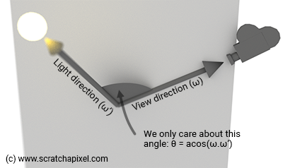

**Figure 2:** the phase function only considers the angle $\theta$ between the light and view direction.

The phase function only depends on the angle between the view and the incoming light direction. This is why it is generally defined in terms of an angle $\theta$ (the Greek letter theta), the angle between the two vectors (and not $\omega$ and $\omega'$). If we take the dot product of the directions $\omega$ (the view direction) and $\omega'$ (the incoming light direction), $\cos(\theta$) spans over the range of [-1, 1] and thus $\theta$ itself spans over the range [0, $\pi$] as shown in the image below.

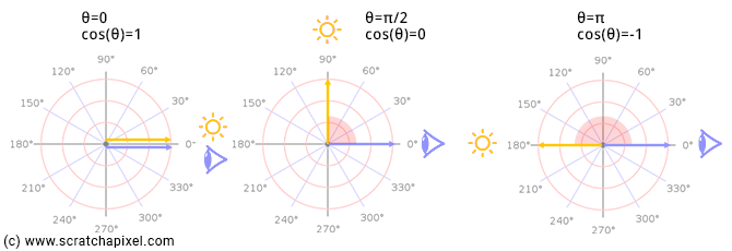
In summary, the phase function tells you how much light is likely to be scattered towards the viewer ($\omega$) for any particular incoming light direction ($\omega'$).

Enough chatting. What do these phase functions look like?

The simplest one is the phase function of isotropic volumes. Because light coming from all sets of directions within the sphere of directions is also equally scattered in all sets of directions over the sphere, uniformly, the phase function (remember its integral over the spherical domain needs to be normalized to 1) simply is:

$$f_p(x, \theta) = { 1 \over {4\pi}}$$

Note that this function is independent of the view and incoming light direction. The $\theta$ angle is there in the function's definition but is not used in the equation itself (on the right-hand side of the equal sign). This is expected since the direction of the out-scattered photon is independent of the incoming light direction (there's no dependency between the two so it has no reason to appear in the equation) and all out-scattered directions are equally likely to be chosen (which is why the equation is a constant). It's not very hard to understand this equation. The area of a sphere is $4\pi$ steradians and so that's basically the surface covered by all our incoming directions if you think of this direction in terms of differential solid angles, and thus the phase function ought to be 1 over $4\pi$ to satisfy the normalization property: the surface covered by all incoming directions divided by $4\pi$ equals 1. This is a good time to mention that the unit of phase functions is 1/sr (sr here stands for steradian).

The phase function for isotropic volumes is quite simple. Let's look at another one called the Henyey-Greenstein phase function. It looks like this:

$$f_p(x, g, \cos\theta) = {1 \over {4\pi}}{{1-g^2}\over{(1 + g^2 - 2g\cos\theta)^{3/2}}}$$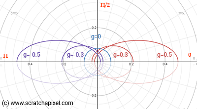

**Figure 3:** plot of the Henyey-Greenstein phase function in the polar coordinate system for different values of the asymmetry factor g (g=0.3, 0.5, 0, -03, -0.5). The angle $\theta$ is defined over the range [0, $\pi$].

It's a little bit more complex indeed. And as you can it has another variable $g$ called the asymmetry factor, where $-1 \leq g \leq 1$. This parameter lets you control whether light is scattered in the forward or backward direction. When $g \gt 0$ light is out-scattered mostly forward. When $g \lt 0$, it is scattered backward. And when $g = 0$, the function equals $1/{4\pi}$, the phase function for isotropic volumes. Figure 3 shows what the function looks like for different values of $g$.

If you want proof that this function is normalized over the sphere of directions, here it is. First, don't forget we need to integrate the function over the sphere of directions (over $4\pi$ steradians) because our directions here say $d\omega$ are defined in terms of differential solid angle. We can write differential solid angles $d\omega$ in terms of $\phi$ (longitude) and $\theta$ (latitude) as explained in the lesson Introduction to Shading. So we get:

$$\int^{2\pi} \Big\{ \int_0^\pi p(\theta) \sin \theta d \theta \Big\} d\phi.$$

Integrating $d\phi$ over $2\pi$ simply gives $2\pi$. So we are left with:

$$2\pi\int_0^{\pi} p(\theta) \sin \theta d \theta.$$

We can write it as a function of $\mu = \cos \theta$, integrating over -1 and 1:

$$2\pi\int_{\mu=-1}^{1} {\color{red}{1 \over {4\pi}}}{{1-g^2}\over{(1 + g^2 - 2g\mu)^{3/2}}} d \mu.$$

We can move the constant in the integral (in red) to the left so we have:

$${1\over 2}\int_{\mu=-1}^{1} {{1-g^2}\over{(1 + g^2 - 2g\mu)^{3/2}}} d \mu.$$

To make this integration, we will use the second fundamental theorem of calculus:

$$\int_a^b f(x) dx = F(b) - F(a).$$

Where $F$ is the anti-derivative of function $f$. So we need to compute the anti-derivative of:

$${{1-g^2}\over{(1 + g^2 - 2g\mu)^{3/2}}}.$$

xx finish this bit xx

Other phase functions exist such as the Schlick, Rayleigh, or Lorenz-Mie scattering phase functions. They've been designed to fit the behavior of different types of particles. For example, it's better to use the Rayleigh function when you attempt to render volumes that are made of tiny particles (smaller than the light wavelength) whereas the Mie function is better for larger particles (dust, water drops, etc.). The Henyey-Greenstein is often used in production rendering, the kind of rendering we do for movies because it's quick to compute (others can be less so) and also simple to sample (see the lesson on Monte Carlo Simulation for example).

Finally, here is what it looks like when we add the Henyey-Greenstein phase function to our code (feel free to implement other functions):

// the Henyey-Greenstein phase function
float phase(const float &g, const float &cos_theta)
{
    float denom = 1 + g * g - 2 * g * cos_theta;
    return 1 / (4 * M_PI) * (1 - g * g) / (denom * sqrtf(denom));
}

vec3 integrate(...)
{
    ...
    float g = 0.8; // asymmetry factor of the phase function
    for (int n = 0; n < ns; ++n) {
        ...
        // In-scattering. Find the distance light travels through the volumetric sphere to the sample.
        // Then use Beer's law to attenuate the light contribution due to in-scattering.
        if (hit_object->intersect(sample_pos, light_dir, isect_vol) && isect_vol.inside) { 
            float cos_theta = ray_dir * light_dir;
            float light_attenuation = exp(-density * isect_vol.t1 * (sigma_a + sigma_s)); 
            result += density * sigma_s * <span style="color: red; font-weight: bold; background-color: rgba(255,0,0,0.1);">phase(g, cos_theta)</span> * light_attenuation * light_color * step_size;
        }
        ...
    }
    ...
}

Note that it looks a lot more like the formal mathematical definition of the in-scattering term provided above.

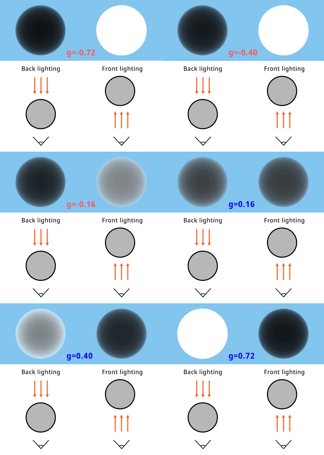
The sequence of images above shows our volume sphere in two different lighting setups with different values for the phase function asymmetry factor $g$. On the left, the light is looking directly at the camera (backlighting). On the right, the light and the camera are pointing straight at the sphere (front lighting).

The Henyey-Greenstein phase function is simple but can offer a good fit to real-world data. You can use a two-lobe phase function for example by combining the result of the function for a value of g = 0.35 with the result for a negative value or higher value of g to achieve a more refined fit. Feel free to experiment. For objects such as clouds or haze, use a high value (around 0.8). Check the reference section at the end of the lesson for some pointers.

Jittering the Sample Positions

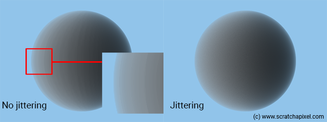
So far, we have always positioned our samples in the middle of the segments. Using regularly spaced samples is like cutting the volume into slices and these slices can lead to some unpleasant banding artifacts as shown in the image above (the effect was artificially exaggerated). To "fix" this problem, we can pick a random position on each segment instead. In other words, samples can be positioned anywhere within the boundaries of a segment (along the camera ray of course). To do so, we will replace these lines:

float t = isect.t0 + step_size * (n + 0.5); 
vec3 sample_pos = ray_orig + t * ray_dir;

With:

float t = isect.t0 + step_size * (n + rand()); 
vec3 sample_pos = ray_orig + t * ray_dir;

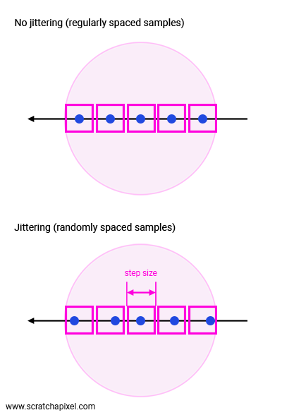
**Figure 4:** to avoid banding artifacts, we can jitter the position of the samples rather than using regularly spaced samples. Samples can be positioned anywhere within the boundaries of a segment.

Where rand() is a function that returns a uniformly distributed number in the range [0,1]. We call this method stochastic sampling.

Stochastic sampling is a Monte Carlo technique in which we sample the function at appropriate non-uniformly spaced locations rather than at regularly spaced locations.

We can't say that this is better (hence the quotes around "fixing the issue"), because we now replace banding with noise, which is a problem on its own. Still, the result is visually more pleasing than banding. You can reduce this noise using more elaborate ways of generating sequences of "random" numbers (see for example quasi Monte-Carlo methods). However, in this version of the lesson, we will skip this topic; an entire book can be written about that (for now, you can find some information on this method in the lesson Monte Carlo in Practice).

Break From the Ray Marching Loop When Opaque (Optimization)

Indeed if the volume's transparency after saying you've marched through half of the distance between t0 and t1 is, for example, lower than 1e-3, you might consider that computing the samples for the remaining half is not necessary (as shown in the adjacent figure). You can do so by just breaking out from the ray-marching loop as soon as you detect that the transparency variable is lower than this minimum threshold (see pseudo-code below). Considering that ray-marching is a rather slow computational method, we should use this optimization; it will save a lot of time particularly when volumetric objects are rather dense (the denser they are, the quicker the transparency drops). We mentioned in the previous chapter that this is one of the reasons why we might prefer the forward over backward integration method.

...
float transparency = 1;
// marching along the ray
for (int n = 0; n < ns; ++ns) {
    ...
    if (transparency < 1e-3)
        break;
}

**Figure 5:** a visualization of the Russian roulette technique. We break out from the ray-marching loop as soon as the transparency gets below a certain threshold but that means that our result is "clamped". How do we fix this problem?

Now you can stop ray-marching when we pass this transparency test and do nothing else however this would be "statistically" wrong. This would somehow introduce some bias in your rendered image. This is more easily understood if you look at figure xx. As you can see, the red line indicates the threshold below which we stop ray-marching. If we do so, we sort of remove the contribution of the volume that's below and beyond the curve (along the x-axis). Sure, the amount is somehow "negligible" and that's why we decided to implement that cutoff solution in the first place, however, if you are a thermonuclear engineer trying to simulate how neutrons move through a plate, this is not acceptable. So how can we still take advantage of this optimization while still satisfying the thermonuclear engineer's expectations?

The method we will be using is called the Russian roulette which we have already talked about already in the lesson dedicated to Monte Carlo methods. The idea is to apply the Russian roulette technique when the transparency value is lower than some threshold for example 1e-3. Then we pick a random number (uniformly distributed) in the range [0, 1] and test whether this random number is greater than 1/d where d is some positive real number (integer but doesn't have to be) greater than 1 (it can be equal to 1 but the test would be useless then). If this is the case, we break out from the loop, otherwise, we continue, however, we multiply the current transparency value by d. The value d here represents the likelihood that we will pass the test. For example for d = 5, the "chances" of the ray-marching loop being terminated would be 4 out of 5.

This makes (hopefully sense). If the random number is lower than 1/d you kill say the photon. It's gone. You can't do anything with it anymore. But in exchange for killing it, we will give more power to the ones that survived the test (increase the transparency value in our case), Inversely proportionally to the likelihood of photons being killed. Here is the idea put into code:

...
float transparency = 1;
// marching along the ray
int d = 2; // the greater the value the more often we will break out from the marching loop
for (int n = 0; n < ns; ++ns) {
    ...
    if (transparency < 1e-3) {
        if (rand() > 1.f / d) // we stop here
            break;
        else
            transparency *= d; // we continue but compensate
   }
}

This is a quick explanation of the Russian roulette technique, which, as already mentioned, is used in Monte Carlo simulation and integration. Please check these lessons for a more detailed explanation if you need to.

Reading Other People's Code!

The first three chapters of this lesson cover what's needed to start rendering volumes. To a point where, if you are confronted with reading other people's code, you should now be able to make sense of what's going on. Let's do this exercise together. We will be using an open-source project called PBRT and looking at its implementation of volume rendering. There should be no secret for you in there any longer.

PBRT is a research/educational project that took more or less the same approach as Scratchapixel: to teach rendering by example. However, PBRT comes as a completely integrated renderer whereas, with Scratchapixel, each technique is implemented in a self-contained example program. Moreover, PBRT was designed for Master/Ph.D. students with the idea that they could use PBRT to implement their research. Most of the equations in PBRT's book are given without much explanation. The book assumes you have the necessary background to read and understand them. Whereas, Scratchapixel aims to teach computer graphics to everyone. We do believe PBRT's book is now online and free for anyone to read. the renderer's source code is available on GitHub.

Besides being a little more complicated than Scratchapixel, it is a reference for students and engineers working in the field. It is still maintained by the authors of the first edition (published in 2004, Scratchapixel started around 2007), Math Pharr, Greg Humphreys, and Pat Hanrahan (more people contributed to the following editions) who keep updating the book and the code with the most recent techniques.

Don't worry if you still find this code overwhelming. It may have taken us years to get familiar with all these concepts. However, we hope that with the explanations given in this lesson, you will be able to follow the broad structure of this code, be able to understand what it does, and get a "now I finally get it" moment).

Spectrum SingleScatteringIntegrator::Li(const Scene *scene, 
    const Renderer *renderer, const RayDifferential &ray, 
    const Sample *sample, RNG &rng, Spectrum *T, 
    MemoryArena &arena) const {

// [comment]
// Find the intersection boundaries (t0, t1) with the volume object. If the ray doesn't
// intersect the volumetric object, then set the transmission to 1 and return 0 as a color.
// [/comment]

    VolumeRegion *vr = scene->volumeRegion;
    float t0, t1;
    if (!vr || !vr->IntersectP(ray, &t0, &t1) || (t1-t0) == 0.f) {
        *T = 1.f;
        return 0.f;
    }

// [comment]
// If we have an intersection. Set the global transmission (transparency) to 1, and the variable
// in which we will store the final color (named Lv here) to 0. Compute the number of samples
// and adjust the step size accordingly.
// [/comment]

    // Do single scattering volume integration in _vr_
    Spectrum Lv(0.);

    // Prepare for volume integration stepping
    int nSamples = Ceil2Int((t1-t0) / stepSize);
    float step = (t1 - t0) / nSamples;
    Spectrum Tr(1.f);
    Point p = ray(t0), pPrev;
    Vector w = -ray.d;
    t0 += sample->oneD[scatterSampleOffset][0] * step;

    // Compute sample patterns for single scattering samples
    float *lightNum = arena.Alloc<float>(nSamples);
    LDShuffleScrambled1D(1, nSamples, lightNum, rng);
    float *lightComp = arena.Alloc<float>(nSamples);
    LDShuffleScrambled1D(1, nSamples, lightComp, rng);
    float *lightPos = arena.Alloc<float>(2*nSamples);
    LDShuffleScrambled2D(1, nSamples, lightPos, rng);
    uint32_t sampOffset = 0;

// [comment]
// Ray-march (forward). This is the main loop, where we will loop over the segments and
// calculate each sample's respective opacity and in-scattering contribution to the
// final volume transparency (Tr) and color (Lv).
// [/comment]

    for (int i = 0; i < nSamples; ++i, t0 += step) {
        // Advance to sample at _t0_ and update _T_

// [comment]
// Update the sample position. Then evaluate the density at that point in the volume.
// We haven't studied this part yet. This is the topic of the next two chapters. For now,
// consider that the variable stepTau is the density variable from our code.
// The sample position is jittered. Then apply Beer's law to attenuate our global
// transmission variable (Tr) with our current sample's opacity.
// [/comment]

        pPrev = p;
        p = ray(t0);
        Ray tauRay(pPrev, p - pPrev, 0.f, 1.f, ray.time, ray.depth);
        Spectrum stepTau = vr->tau(tauRay,
            .5f * stepSize, rng.RandomFloat());
        Tr *= Exp(-stepTau);

// [comment]
// Apply the russian-roulette technique.
// [/comment]

        // Possibly terminate ray marching if transmittance is small
        if (Tr.y() < 1e-3) {
            const float continueProb = .5f;
            if (rng.RandomFloat() > continueProb) {
                Tr = 0.f;
                break;
            }
            Tr /= continueProb;
        }

// [comment]
// We survived. Let's compute the in-scattering contribution for that sample. Normally
// one could calculate the contribution of each light in the scene. However, this code
// uses a different technique. It selects one light randomly and calculates the contribution
// of that one single light instead. This is another example of Monte Carlo integration.
// Don't worry too much about this for now. We will study this in a future lesson.
// [/comment]

        // Compute single-scattering source term at _p_
        Lv += Tr * vr->Lve(p, w, ray.time);
        Spectrum ss = vr->sigma_s(p, w, ray.time);
        if (!ss.IsBlack() && scene->lights.size() > 0) {
            int nLights = scene->lights.size();
            int ln = min(Floor2Int(lightNum[sampOffset] * nLights),
                nLights-1);
            Light *light = scene->lights[ln];
            // Add contribution of _light_ due to scattering at _p_
            float pdf;
            VisibilityTester vis;
            Vector wo;
            LightSample ls(lightComp[sampOffset], lightPos[2*sampOffset],
                lightPos[2*sampOffset+1]);

// [comment]
// Calculate the light color (color * intensity, etc.)
// [/comment]

            Spectrum L = light->Sample_L(p, 0.f, ls, ray.time, 
                &wo, &pdf, &vis);
            
            if (!L.IsBlack() && pdf > 0.f && vis.Unoccluded(scene)) {

// [comment]
// Multiply the light color by the light transmission value (how much light is left
// after it has traveled through the volume to the sample point). Beer's law is
// applied in the Transmittance function (code not shown here but you can check
// PBRT source code).
// [/comment]

                Spectrum Ld = L * vis.Transmittance(scene, 
                    renderer, NULL, rng, arena);

// [comment]
// Then add the in-scattering contribution to our final color. Note here that we
// multiply by all the right terms: Tr (the volume current transparency value),
// ss (the scattering term), vr->p (the phase function), Ld (the light contribution,
// the Li(x) term). Forget about the other terms, they have to do with the Monte Carlo
// integration method we talked about earlier. Note: we don't multiply by the step size
// here because it's done at the very end. Outside the ray-marching loop.
// [/comment]

                Lv += Tr * ss * vr->p(p, w, -wo, ray.time) * Ld * 
                    float(nLights) / pdf;
            }
        }
        ++sampOffset;
    }
    *T = Tr;

// [comment]
// Finally multiply the final color by the step size. In our code, we've done it in the
// ray-marching loop for clarity. But for optimization, you might want to do it at
// the very end which is what they decided to do here.
// [/comment]

    return Lv * step;
}

Source Code

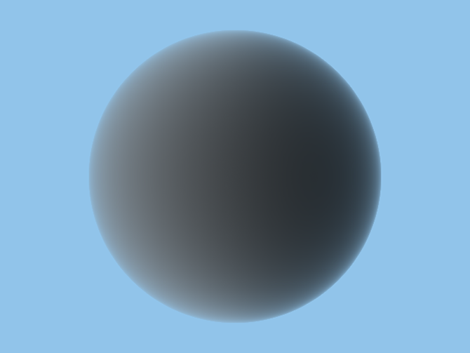
The source code for this chapter is available at the end of the lesson. And it should produce the following image. Note that in this version of the code the light color has higher values. The phase function introduces a division by $4\pi$ which is the reason why we now need to increase the light color a lot.

Exercises

You can test that the russian roulette method works?
Make the code work for an arbitrary number of lights?
Move the camera around using matrices. Deform the volume sphere using matrices as well (try to squeeze/squash the sphere). You can find some clues on how to do that in this lesson: Transform Objects using Matrices.
Make it work with the camera inside the volume.
Replace the sphere with a cube.
Add a timer, to measure how slow volume rendering is. This will be most noticeable in the next chapter.

What's next?

Congratulation if you made it that far. You graduated and Scratchapixel is delivering you a virtual certificate with honors. The core of how these algorithm works has been covered. The remaining chapters are more about using what we have learned and built so far, to finally have some fun and make some cool images. Finally, in the last chapter, we will take everything we have learned so far, and see how it translates into the actual equations used to describe the flux of light energy as it travels through and interacts with a participating medium (air, smoke, cloud, water, etc.)