Mathematical Foundations of Monte Carlo Methods

Probability Distribution: Part 2

Reading time: 3 mins.

In chapter 2, we have mentioned the normal (or gaussian) probability distribution. We now have the knowledge needed to introduce and understand its equation. Why study the normal distribution? This distribution is very common in nature. For example, the adult height in any adult given population generally follows (more or less) a normal distribution. We will see it appearing in the next chapter as well.

If you reproduce these curves for yourself, you will probably get a better sense of what the parameters of the equation do. You can use Grapher on Mac and Gnuplot on Linux.

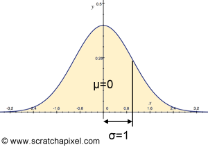
The gaussian or normal distribution has a typical bell-shaped curve (see figure 1). The equation for this distribution is a bit complex:

$$p(x) = \mathcal{N}(\mu, \sigma) = {\dfrac{1}{\sigma \sqrt {2 \pi} } } e^{-{\dfrac{(x -\mu)^2}{2\sigma^2}}}.$$

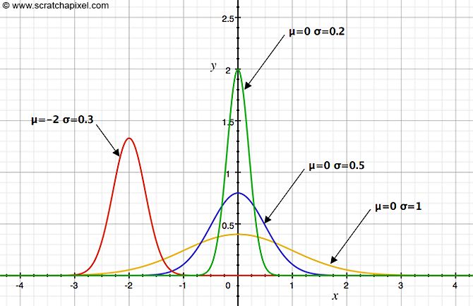
**Figure 1:** a normal distribution with standard deviation ($\sigma = 1$) and expectation ($\mu = 0$).

You should already be familiar with the $\sigma$ term (the greek letter sigma) which is the distribution's standard deviation (see the previous chapter if you need a refresher on what the standard deviation is). The term $\mu$ (the greek letter mu) is the distribution's expectation (a concept we have also introduced in the previous chapter). Note that the curve is symmetrical around $\mu$. By changing the value of these parameters we can obtain all sorts of bell-shaped distributions as pictured in figure 2\. The normal distribution function is generally denoted $\mathcal{N}(\mu, \sigma)$ since mean and variance are the two parameters of the model. $\mathcal{N}(0,1)$ is called the standard normal distribution (figure 1).

Advanced: add in a future revision of the lesson to show that the expected value of the standard normal distribution is 0, the area under the curve is 1 and the standard deviation is 1\. Note in the figure below that when the standard deviation is smaller the curve is higher. The area under the curve is 1 no matter which standard deviation you chose.

**Figure 2:** example of gaussian distribution for different values of the standart deviation ($\sigma$) and different values of the mean ($\mu$).

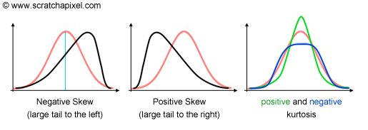
If you read more about statistics you may come across the terms skew and kurtosis. In the image above we have drawn a normal distribution in red (with a standard deviation of 2 and a mean of 5). When the curve is perfectly symmetrical around the mean (the vertical cyan line) then we say that the skew of the distribution is 0. When the distribution has a larger tail to the left, the skew is negative (and the skew is positive when the tail is larger to the right). The term kurtosis designates how pointy or smooth the curve is compared to a normal distribution (right). A curve that is narrower than the normal distribution is said to have a positive kurtosis. These are not so important (especially in computer graphics) but these two parameters will help us in the next chapter to compare how close our distribution of data is to a "perfect" normal distribution.

In the next chapter, we will learn about the concepts of PDF (probability density function) which is derived from the concept of a probability distribution, and CDF (cumulative distribution function). These two concepts are very important in computer graphics.