Mathematical Foundations of Monte Carlo Methods

Variance and Standard Deviation

Variance and Standard Deviation

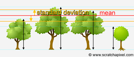
Imagine that you measure the height of a certain number of trees which have grown for the same amount of time. Most trees have probably all grown more or less the same way thus after let's say 10 years, you expect them to have all more or less the same height, however some trees may have a much smaller height than what you would expect. However saying that a tree is smaller than you would expect requires that you can define what's you expect the average height of a 10 years old tree to be in the first place, and of course, since trees are unlikely to have exactly the same height, it requires that you also define an interval within which you accept some level of variation from this average. Only then can a tree whose height does not fall within this interval (centred around the average tree height) be considered as unusually taller or unusually smaller than the rest of the trees (this can be very useful in statistics to define for example whether a particular individual from a given population and of a given age, follows a normal growth rate). Computing the average tree height is simple: you just add up all the trees height and divide the resulting number by the total number of trees. But how do we compute the range of variation within which a tree height can be considered normal or not? This is where variance and standard deviation come into play. Standard deviation is simply the square root of variance, thus we will just concentrate on variance for now. Technically variance is defined as the expected value of the square difference between the outcome of the experiment (let's say the height of each tree) and its expected value (in the tree example, the tree average height). Variance can be expressed as:

We know that \(E[X] = \sum_{i=1} p_i x_i\) thus if we set \(x = (a - b)^2\) we get \(E[(a-b)^2] = \sum_{i=1} (a-b)_i^2 p_i\) where in our example, \((a-b)^2 = (x - E[X])^2\). That is really all there is to the equation above. The symbol \(\sigma\) is the greek letter sigma (and you can read variance as "sigma squared"). The definition of variance is hard to make sense of but the concept is actually simple. For instance you take the difference between the height of the first tree and the expected value which in this example is the average tree height, you take the square of this number, repeat this process for all the remaining trees and add up the numbers. This gives you the variance for the height of the trees. And taking the square root of this number gives you the standard deviation:

Since we are in the realm of statistics, large numbers and probability here, this number can be interpreted as being an acceptable variation of the height above or below the average value within which you can consider the height of any tree to be a valid representation of the overall tree population's height.

This can also be seen as some average distance between the points of a set of data points, where the data set in our example is our collection of trees (see the example below) or put it differently, the average distance from the mean of all the samples. The expected value is additive, \(E[f+g] = E[f] + E[g]\) and the expected value of a constant is that constant (\(E[c] =c \)) thus if we write \(\mu = E[X]\) (where \(\mu\), the greek letter mu, in statistics, designates the population mean or population expected value (see previous chapter for more information on this and expected value properties). In our tree example for instance, this is the average tree height calculated from summing up the the height of all the trees and dividing the resulting number by the total number of trees). The expression for variance can be expanded into:

This formulation is useful in computing because as you go through the elements to compute the population mean you can also compute the left term (the sum). And the end of this process, you are left with subtracting the population mean form the sum of the squared observations (see the chapter on sampling distribution for an example). Of course the technique works whether you consider all the elements in the population or just the elements from a sample of certain size. When you consider the entire population the term on the right is the population mean. If you work from a sample, it would be more accurate to call the term on the right the sample mean (which, if the sample size is large enough, is also the expected value of the random variable). If all random variables have the same probability then note that we can also write (we assume here that we work from a sample of size \(n\)):

Where \(n\) is the total number of random variables being considered in the calculation of the sample mean.

Properties of Variance

Properties of variance are quite important to understand or interpret some of the techniques we will introduce next. It is important to know wat they are. Not susprisingly they are very similar to the expected value properties:

• If \(Pr(X = c) = 1\), then \(Var(X) = 0\). This requires a short explanation. If we have an experiment that is always returning the exact same outcome (this outcome's probability is 1), thus the variance is simply 0. More formally if there exists a constant \(c\) such that \(Pr(X = c) = 1\), then \(E[c] = c\) (see expectations properties), and \(Pr[(X - c)^2 = 0] = 1\). Therefore \(Var(X) = E[(X-c)^2] = 0\).

• If we note \(Y = aX + b\) then $$Var(Y) = a^2 Var(X).$$If \(E[X] = \mu\), then \(E[Y] = a\mu + b\) (see expectations' properties).

  Thus we can write:

  $$ \begin{array}{l} Var(Y) &=& E[(aX + b - a\mu -b)^2] = E[(aX - a\mu)^2]\\ &=&a^2E[(X-\mu)^2]=a^2Var(X). \end{array} $$

  Note that \(Var(X + b) = Var(X)\). Again, this is easy to understand. Shifting the height of all the trees by the same amount won't change the population's variance. The expected value will change but not variance.

• If \(X_1, ..., X_n\) are independent random variables, then:

  $$Var(X_1 + ... + X_n) = Var(X_1) + ... + Var(X_n).$$

  Let's prove this properly using two random variables \(X_1\) and \(X_2\)) (\(n = 2\)). If \(E[X_1] = \mu_1\) and \(E[X_2] = \mu_2\), then:

  $$E[X_1 + X_2] = \mu_1 + \mu_2.$$

  Therefore:

  $$ \begin{array}{l} Var(X_1 + X_2) &=& E[(X_1 + X_2 + \mu_1 + \mu_2)^2]\\ &=&E[(X_1-\mu_1)^2 + (X_2 - \mu_2)^2 + 2(X_1 - \mu_1)(X_2 - \mu_2)]\\ &=&Var(X_1) + Var(X_2) + 2E[(X_1-\mu_1)(X_2 - \mu_2)]. \end{array} $$

  \(X_1\) and \(X_2\) are independent, thus:

  $$ \begin{array}{l} E[(X_1-\mu_1)(X_2-\mu_2)] &=& E[(X_1-\mu_1)]E[(X_2 - \mu_2)]\\ &=&(\mu_1 - \mu_1)(\mu_2 - \mu_2)\\ &=&0. \end{array} $$

  Finally, we are left with:

  $$Var(X_1 + X_2) = Var(X_1) + Var(X_2).$$