Sampling Distribution
Reading time: 34 mins.Read this chapter carefully. It describes the most important concepts for understanding the Monte Carlo method. Because there is so much to read in this chapter already, a lot of the mathematical proofs for the equations presented in this chapter will be provided in the next chapter.
Sampling Distribution: Statistic from Statistics
It is not possible to calculate the population mean of an infinite population (such a population can be thought of as the outcome of an infinite number of coin tosses. Of course this concept is only theoretical and such a population has only a hypothetical existence). Even when the population is finite but very large, computing a mean can reveal itself to be an impractical task. When facing either one of these situations, what we can do instead is draw samples from the population (where each of these samples can be seen as a random variable) and divide the sum of these drawn random variables by the number of samples to get what we call a sample mean \(\bar X\). What this number gives is an estimation (not an approximation) of the population mean \(\mu\). We have already introduced these two concepts in the previous chapter.
In statistics when some characteristic of a given population can be calculated using all the elements or items in this population, we say that the resulting value is a parameter of the population. The population mean for example is a population parameter that is used to define the average value of a quantity. Parameters are fixed values. On the other hand, when we use samples to get an estimation of a population parameter we say that the value resulting from the samples is a statistic. Parameters are often given greek letters (such as \(\sigma\)) while statistics are usually given roman letters (e.g. \(S\)). Note that because it is possible to draw more than one sample from a given population, the value of that statistic is likely to vary from sample to sample.
The way we calculate things such as the mean or variance depends on whether we use all the elements of the population or just samples from the population. The following tables help to compare the difference between the two cases:
Population (parameter) |
|---|
\(\bar x \approx \mu \) |
A parameter is a value, usually unknown (and which therefore has to be estimated), used to represent a certain population characteristic. For example, the population mean is a parameter that is often used to indicate the average value of a quantity. |
\(N\) is the total size of the population (e.g. the total population of a country). |
Mean |
\(\mu = \dfrac{\sum_{i=1}^N {x_i}}{N}\) |
Variance |
\(\sigma^2 = \dfrac{\sum_{i=1}^N {(x_i - \mu)^2}}{N} = \dfrac{\sum_{i=1}^N x_i}{N} - \mu^2\) |
Sample (statistics) |
|---|
\(\bar x \approx \mu \) |
A statistic is a quantity that is calculated from a sample of data. It is used to give information about unknown values in the corresponding population. For example, the average of the data in a sample is used to give information about the overall average in the population from which that sample was drawn. |
\(n\) is the size of the sample (e.g. the number of times we toss the coin). |
Mean |
\(\bar X = \dfrac{\sum_{i=1}^n x_i }{n}\) |
Variance |
\(S_n^2 = \dfrac{\sum_{i=1}^n (x_i - \bar X)^2 }{n} = \dfrac{\sum_{i=1}^n x_i}{n} - \bar X^2\) |
Note that the variance of a statistic is denoted \(S_n^2\) (where the subscript n denotes the number of elements drawn from the population) to differentiate it from the population variance \(\sigma^2\). The second formulation for the variance is helpful because, from a programming point of view, you can use it to compute the variance as you draw elements from the population (rather than waiting until you have all samples). Now that we have established the distinction between the two cases and their relationship (a statistic is an estimation of a population's parameter) let's pursue a practical example. To make the demonstration easier, we wrote a C++ program (see source code below) generating a population of elements defined by a parameter which is an integer between 0 to 20 (this is similar to the experiment with cards labeled with numbers). To generate this population, we arbitrarily pick up a number between 1 and 50 for each value contained in the range [0,20]. This number represents the number of elements in the population having a particular value (either 0, 1, 2, etc. up to 20). The size of the population is the sum of these numbers. The parameters (population size, population mean, and variance) of this population are summarized in the next table:
Population Size |
Population Mean |
Population Variance |
|---|---|---|
572 |
8.970280 |
35.476387 |
The rest of the program will sample this population 1000 times, where the size of the sample (the number of elements drawn from the population to calculate the sample mean and the sample variance) will vary from 2 to 20; this will help us to see how differently the sampling technique works for low and high number of samples. We randomly select a sample size of n and then draw n samples from the population where for each draw, we first randomly select an item from the population (any random number between 1 and the population size).
The process by which we find out the value held by this item is a bit unusual. We incrementally remove the number of items holding a particular value (starting for the group of items holding the value 0, then 1, etc.) from the item index, and we break from this loop, as soon as the item index gets lower than 0.
int item_index = pick_item_distr(rng), k;
for (k = 0; k <= MAX_NUM; ++k) {
    item_index -= population[k];
    if (item_index < 0) break;
}
The value of k in the code when we break from that loop is the value held by the chosen element. This technique works because the index of the drawn element is randomly chosen (i.e. the likelihood of choosing an element in the group of 1s, is the same as choosing an element in the group of 2s, 3s,... or 20s).

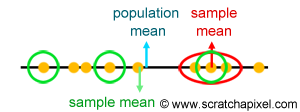
As the elements are drawn from the population we update the variables used for computing the sample mean and the sample variance. At the end of this process, we get 1000 samples (to start with) with their associated sample mean and variance. Plotting these results will help us to make some interesting observations about the process of drawing samples from a population. Note that in the graph (figure 1), samples with a small size are drawn in red, while samples with a large size are drawn in blue (the sample color is interpolated between red and blue when its size is somewhere between 2 and 20). The green spot in the figure indicates the point on the graph where the population parameters (the mean and the variance) coincide. Any sample which is close to this point can be considered as providing a good estimate of the population mean and variance. The further away a sample is from this point (in either direction), the poorer the estimation.
Here is the source code of the program used to generate the data in Figure 1.
#include <random>
#include <cstdlib>
#include <cstdio>

static const int MAX_NUM = 20;   //items in the population are numbered (number between 0 and 20)
static const int MAX_FREQ = 50;  //number of items holding a particular number varies between 1 and 50

int main(int argc, char **argv)
{
    int minSampples = atoi(argv[1]);  //minimum sample size
    int maxSampples = atoi(argv[2]);  //maximum sample size
    std::mt19937 rng;
    int population[MAX_NUM + 1];
    int popSize = 0;
    float popMean = 0;
    float popVar = 0;
    static const int numSamples = 1000;

    rng.seed(17);

    // creation population
    std::uniform_int_distribution<uint32_t> distr(1,MAX_FREQ);

    for (int i = 0; i <= MAX_NUM; ++i) {
        population[i] = distr(rng);
        popSize += population[i];
        popMean += population[i] * i;  //prob * x_i
        popVar += population[i] * i * i;  //prob * x_i^2
    }

    popMean /= popSize;
    popVar /= popSize;
    popVar -= popMean * popMean;
    fprintf(stderr, "size %d mean %f var %f\n", popSize, popMean, popVar);
    std::uniform_int_distribution<uint32_t> n_samples_distr(minSampples, maxSampples);
    std::uniform_int_distribution<uint32_t> pick_item_distr(0, popSize - 1);

    float expectedValueMean = 0, varianceMean = 0;
    // now that we have some data and stats to work with sample it
    for (int i = 0; i < numSamples; ++i) {
        int n = n_samples_distr(rng);  //sample size
        float sample_mean = 0, sample_variance = 0;
        // draw samples from the population and compute stats
        for (int j = 0; j < n; ++j) {
            int item_index = pick_item_distr(rng), k;
            for (k = 0; k <= MAX_NUM; ++k) {
                item_index -= population[k];
                if (item_index < 0) break;

            }
            // k is the value we picked up from the population,
            // this is the outcome of a number between [0:20]
            sample_mean += k;
            sample_variance += k * k;
        }
        sample_mean /= n;
        sample_variance /= n;
        sample_variance -= sample_mean * sample_mean;

        float c1[3] = { 1, 0, 0 };
        float c2[3] = { 0, 0, 1 };
        float t = (n - minSampples) / (float)(maxSampples - minSampples);
        float r = c1[0] * (1 - t) + c2[0] * t;
        float g = c1[1] * (1 - t) + c2[1] * t;
        float b = c1[2] * (1 - t) + c2[2] * t;
        printf("sample mean: %f sample variance: %f col: %f %f %f;\n", sample_mean, sample_variance, r, g, b);
    }

    return 0;
}

What observations can we make from looking at this graph? First, note that the graph can be read along the abscissa (x) and ordinates (y) axis. Any sample close to the sample mean line (the vertical cyan line) can be considered as providing a good estimate of the population mean. Any sample close to the population variance line (the horizontal cyan line) provides a good estimation of the population variance. However, truly "good" samples are samples that are close to both lines. We have illustrated this in figure 1 with a yellow shape showing a cluster of samples around the green dot which can be considered good samples because they are in reasonable proximity to these two parameters (if you are interested in this topic, read about confidence interval). Note also that most samples in this cluster are blue but not all of them are (there is still a small portion of red or reddish samples). This tells us that the bigger the sample size, the more likely we are to come up with an estimate converging to the population's parameters. Note though that we said, "we are more likely". We didn't say the bigger the sample size the better the estimate. This is capturing the difference (however subtle and philosophical) there is between statistics and the concept of approximation. In statistics, there is always a possibility (even if very small) that the values given by a sample will be the same as the population's parameters. However unlikely, this chance exist no matter how big (or small) the sample size. However, a sample whose size is very small is more likely to provide an estimate which is way off, than a sample whose size is much larger even though the sample estimate is more likely to converge to the population's parameters.
Note 1: indeed, by the law of large numbers (which we have presented in chapter 2), the sample averages converge in probability and "almost" surely to the expected value \(\mu\) as n approaches infinity.
Note how we used "almost" in the previous definition. We can't predict for sure that it will converge, but we can say that the probability that it will, gets higher as the sample size increases. It is all about probabilities. Figure 2 shows what happens to the "quality" of the samples as the sample size increases. Samples are still distributed around the population mean and variance but the cluster of samples shrank indicating indeed that the quality of the estimation is on average better than what we had in figure 1\. In other words, the cluster gets smaller as n increases (indicating an overall improvement in the quality of the estimation), or to word it differently, you can say that the statistics get more and more concentrated around some value as \(n\) increases. From there we can ask two questions? What that value is and what happens to these statistics as \(n\) approaches infinity? But we already gave the answers to these questions when we introduced to Law of Large Numbers. The value is the population mean itself and the sample mean approaches this population mean as \(n\) approaches infinity. Remember this definition from the chapter on the Expected Value:
$$ \begin{array}{l} \lim_{n \rightarrow \infty} \text{ Pr }(|\bar X - \mu| < \epsilon) = 1 \\ \bar X \rightarrow \mu. \end{array} $$
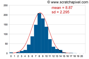
As you can see in figure 3 the population generated by our program has an arbitrary distribution. This population is not distributed according to any particular probability distribution, and especially not a normal distribution. The reason why we made this choice will become clear very soon. Because the distribution is discrete and finite, this population of course has a well-defined mean and variance which we already computed above. What we are going to do now is take a sample of size \(n\) from this population, compute its sample mean and repeat this experiment 1000 times. The sample mean value will be rounded off to the nearest integer value (so that it takes any integer value between 0 and 20). At the end of the process, we will count the number of samples whose means are either 0, 1 or 2, ... up to 20. Figure 4 shows the results. Quite remarkably, as you can see, the distribution of samples follows a normal distribution. This is not the distribution of cards here that we are looking at but the distribution of samples. Be sure to understand that difference quite clearly. It is a distribution of statistics. Note also that this is not a perfect normal distribution (you now understand why we have been very specific about this in the previous chapter) because clearly, there is some difference between the results and a perfect normal distribution (curve in red). In conclusion, even though the distribution of the population is arbitrary, the distribution of samples or statistics is not (but it converges in distribution to the normal distribution. We will come back to this idea later).
Question from a reader: on which basis do you claim that the sampling distribution is not a perfect normal distribution? And how do you get the curve to fit your data (the red curve in figure 4)? We know that a normal distribution is defined by a mathematical equation and two parameters which are the mean and the standard deviation (check the previous chapter). From a computing point of view, it is possible to measure the skew and the kurtosis of our sampling distribution (but we not showing how in this version of the lesson). If any of these two parameters are non zero then we know for sure that our sampling distribution is not a perfect normal distribution (check the previous chapter for an explanation of these two terms). As for the second question, it is possible to compute the expected value of the samples and their standard deviation (we show how below) and from these numbers, we can draw a curve such as the one you see in Figure 4. Keep in mind that this curve is not meaningful. What you care about are the samples and their sampling distribution. You can interpret the curve as showing the overall tendency of the sampling distribution.
The following code snippet shows the changes we made to our code to compute the data for the chart in figure 4.
int main(int argc, char **argv)
{
    ...

    int meansCount[MAX_NUM + 1];
    for (int i = 0; i <= MAX_NUM; ++i) meansCount[i] = 0;

    // now that we have some data and stats to work with sample it
    for (int i = 0; i < numSamples; ++i) {
        ...
        meansCount[(int)sample_mean]++;
    }

    for (int i = 0; i <= MAX_NUM; ++i) printf("%d %d\n", i, meansCount[i]);
    ...
}
We have repeated many times that the sample means and the sample variance are random variables of their own (each sample is likely to have a different value than the others), and thus like any other random variables, we can study their probability distribution. In other words, instead of studying for example how the height (the property) of all adults from a given country (the population) is distributed, we take samples from this population to estimate the population's average height and look at how these samples are distributed with regards to each other. In statistics, the distribution of samples (or statistics) is called a sampling distribution. Similarly to the case of population distribution, sampling distributions can be defined using models (i.e. probability distributions). It defines how all possible samples are distributed for a given population and samples of a given size.
Note 2: the sampling distribution of a statistic is the distribution of that statistic, considered as a random variable when derived from a random sample of size n. In other words, the sampling distribution of the mean is a distribution of sample means.
Keep in mind that a statistic on its own is a function of some random variables, and consequently is itself a random variable. As with all other random variables it hence has a distribution. That distribution is what we call the sampling distribution of the statistic \(\bar X\). The values that a statistic can have and how likely it is to take on any of these values are defined by the statistic's probability distribution.
An important point to make from these definitions is that if you know the sampling distribution of some statistic \(\bar X\) then you can find out what the probability or how likely \(\bar X\) will take on some values before observing the data.
The next concept is an extension of the technique we have been using so far. Remember how we learned to calculate an expected value in chapter 1? In the case of discrete random variables (the concept is the same for continuous r.v. but the concept is easier to describe with discrete r.v.), we know the expected value or mean is nothing more than the sum of each outcome weighted by its probability.
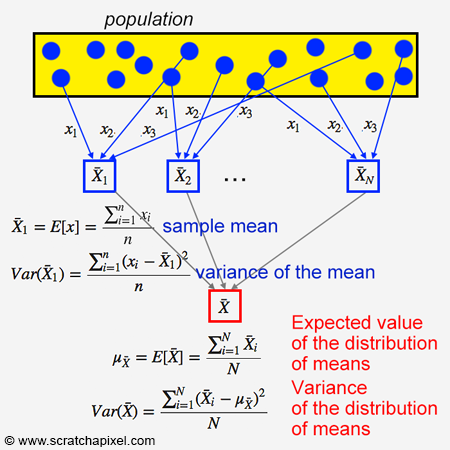
Note 3: just as the population can be described with parameters such as the mean, so can the sampling distribution. In other words, we can apply to samples or statistics the same method for computing a mean as the method we used to calculate the mean of random variables. When applied to samples, the resulting value is called the expected value of the distribution of mean and can be defined as:
$\mu_{\bar X} = E(\bar X) = \sum_{i=1}^n p_i \bar X_i,$
where \(p_i\) is the probability associated with the sample mean \(\bar X_i\) and where these probabilities are themselves distributed according to sampling distribution. When the samples are drawn with the same probability (i.e. uniform distribution) the probability is just \(1 \over n\) where \(n\) here stands for the number of samples or statistics (not the sample size).
For reasons beyond the scope of this lesson, \(\mu_{\bar X} \) can not be considered the same thing as a mean (because as the sample size approaches infinity this value is undefined), however, it can be interpreted or seen as something similar to it. This expected value of the distribution of means can be seen somehow as a weighted average of a finite number of sample means. Not the average, but the weighted average where the weight is the frequency (or probability) of each possible outcome:
$$E(\bar X) = \sum_{i=1}^n w_i \bar X_i.$$This is the same equation as before, but we replaced \(p_i\) with \(w_i\); in this context though, the two terms are synonymous.
It can be proven that the expected value of the distribution of means \(\mu_{\bar X} \) is equal to the population mean \(\mu\): \(\mu_{\bar X} = \mu\). The proof of this equality can be found at the end of this chapter (see Properties of Sample Mean). However, let's just say for now that in statistics, when the expected value of a statistic (such as \(\mu_{\bar X}\)) equals a population parameter, the statistic itself is said to be an unbiased estimator of that parameter. For example, we could say that \(\bar X\) is an unbiased estimator of \(\mu\). Again this important concept will be reviewed in detail in the next chapter. We will also show in the chapter on Monte Carlo, that Monte Carlo is an (unbiased) estimator.

If now increase the sample size (i.e. increase \(n\)) then the samples are more likely to give a better estimate of the population mean (we have already illustrated this result in figure 2). Not all samples are close to the mean, but generally the higher the sample size (\(n\)), the closer the samples are to the mean. The distribution of samples has the shape of a normal distribution as in the previous case, but if you compare the graphs from Figures 3 and 4 you can see that the second distribution is tighter than the first one. As \(n\) increases, you get closer to using all the elements from the population for estimating the mean, thus logically the sample means are more likely on average, to be close to the population mean (or to say it another way, the chance of having sample means away from the population mean is lower). This experiment shows something similar to what we have already looked at in Figures 1 and 2 (check note 1 again) which is that the higher the sample size, the more likely we are in probability to converge to the true mean (i.e. the population mean). We could easily confirm this experimentally by looking at the way the expected value of the distribution of means \(\mu_{\bar X}\) (as well as its associated standard deviation \(\sigma_{\bar X}\)) varies as we increase the sample size. We should expect the expected of the sample means \(\mu_{\bar X}\) to converge to the population mean \(\mu\) and the normal distribution (measured in terms of its standard deviation) to keep becoming tighter as the sample size increases. Here are the changes we made to the code to compute these two variables named expectedValueDistrMeans (the equivalent of \(\mu_{\bar X}\) and varianceDistrMeans (the equivalent of \(\sigma_{\bar X}\)). In this version of the code, each sample has the same sample size (line 6) and we also increased the total number of samples (line 4) from the population to improve the robustness of the estimation (we went from 1000 to 1000 statistics or samples):
int main(int argc, char **argv)
{
    ...
    static const int numSamples = 10000;
    ...
    float expectedValueDistrMeans = 0, varianceDistrMeans = 0;
    for (int i = 0; i < numSamples; ++i) {
        int n = atoi(argv[1]); // fix sample size
        float sample_mean = 0, sample_variance = 0;
        for (int j = 0; j < n; ++j) {
            ...
        }
        sample_mean /= n;
        sample_variance /= n;
        sample_variance -= sample_mean * sample_mean;
        meansCount[(int)(sample_mean)]++;

        expectedValueDistrMeans += sample_mean;
        varianceDistrMeans += sample_mean * sample_mean;
    }
    expectedValueDistrMeans /= numSamples;
    varianceDistrMeans /= numSamples;
    varianceDistrMeans -= expectedValueDistrMeans * expectedValueDistrMeans;
    fprintf(stderr, "Expected Value of the Mean %f Standard Deviation %f\n", expectedValueDistrMeans, sqrt(varianceDistrMeans));

    return 0;
}
Are you lost? Some readers told us that at this point they tend to be lost. They don't understand what we try to calculate anymore. This is generally the problem in statistics when you get to this point because the names themselves tend to become confusing. For example, it might take you some time to understand what we refer to when we speak of the mean of the sampling distribution of the means. To clarify things, we came up with the following diagram:
We ran the program several times each time increasing the sample size by 2\. The following table shows the results (keep in mind that the population mean which we compute in the program is 8.970280):
Sample Size (n) |
Mean \(\mu_{\bar X}\) |
Standard Deviation \(\sigma_{\bar X}\) |
|---|---|---|
2 |
8.9289 |
4.275 |
4 |
8.9417 |
3.014 |
8 |
8.9559 |
2.130 |
16 |
8.9608 |
1.512 |
32 |
8.9658 |
1.074 |
... |
... |
... |
16384 |
8.9703 |
0.050 |
First, the data seems to confirm the theory: as the sample size increases, the mean of all our samples (\(\mu_{\bar X}\)) approaches the population mean (which is 8.970280). Furthermore, the standard deviation of the distribution of means \(\sigma_{\bar X}\) decreases as expected (you can visualize this as the curve of the normal distribution becomes narrower). Thus as stated before, as \(n\) approaches infinity, the sampling distribution turns into a perfect normal distribution of mean \(\mu\) (the population mean) and standard deviation 0: \(N(\mu, 0)\). We say that the random sequence of random variables \(X_1, ... X_n\), converges in distribution to a normal distribution.
Try to connect the concept of convergence in distribution with the concept of convergence in probability which we have talked about in the chapter on expected value.
This is important because mathematicians like to have the proof that eventually the mean of the samples \(\mu_{\bar X}\) and the population mean \(\mu\) are the same and that the method is thus valid (from a theoretical point of view because obviously in practice, the infinitely large sample size is impossible). In other words, we can write (and we also checked this result experimentally) that:
$$\mu_{\bar X} = E[\bar X] = \mu.$$And if you don't care so much about the mathematics and just want to understand how this applies to you (and the field of rendering) you can just see this as "your estimation becomes better as you keep taking samples (i.e. as \(n\) increases)". Eventually, you have so many samples, that your estimation and the value of what you are trying to estimate are very close to each other and even the same in theory when you have an infinity of these samples. That's all it "means".
Let's now talk about something that is certainly of great importance in statistics but even more in rendering (at last something useful to us). If you look at the table again you may have noticed that the difference between the expected value of the distribution of means when N=2 and N=16 are greater (8.9608 - 8.9289 = 0.0319) than the difference for the expected value when N=32 and N=16384 (8.9703 - 8.9658 = 0.0045). In other words, the estimation when going from 32 to 16384 samples is only a fraction better (the exact value is 0.0319/0.0045) than when going from 2 to 16 samples!
When you keep increasing the sample size \(n\) and we will prove this relationship at the end of the chapter, the variance of the distribution of means decreases according to the following equation:
$\sigma_{\bar X} = {\dfrac{\sigma}{\sqrt{n}}}.$
Where \(\sigma\) is the standard deviation of the population and \(n\) is the sample size. In other words, the rate at which the standard deviation of the distribution of means (which you can interpret as the error in the estimation of the population mean, in fact in statistics, the standard deviation of the distribution of means \(\sigma_{\bar X}\) is called the standard error) decreases with the number of samples (\(\sqrt{n}\)) and is non-linear (the square root operator is a nonlinear operator). We can say that the rate of convergence is \(O(\sqrt{n})\) if you wish to use the big O notation (you can read this as "the algorithm's performance is directly proportional to the square root of n"). Note that the variance \(\sigma_{\bar X}^2\) also known in statistics as the Mean Squared Error (MSE), varies linearly with \(n\) since variance is the square root of standard deviation.
The consequence of this relationship, is that four times more samples are needed to decrease the error of the estimation by half.
We will come back to this observation when we get to the chapter on the Monte Carlo method.

The following sequence of results helps to understand the "four times more samples are needed to decrease the error of the estimation by half" better. Imagine that the standard deviation of the population is 1 to start with and that you start with a sample size of 4, thus your standard error is \(error = 1/\sqrt{4} = 0.5\). Now if you want to decrease the error by 2 you need 4 times as many samples, that is 16 samples. Let's check: \(error = 1/\sqrt{16}=0.25\) which is correct. And again if you want to decrease this error by half one more time, you need 4 times 16 samples which are 64 samples: \(error = 1/\sqrt{64}=0.125\). Note that the processing time increases linearly with respect to the sample size, thus quadrupling the number of samples increases the processing time by four (assuming a linear relationship between the number of samples and the processing time, which is a reasonable assumption). This should start giving you intuition as to why Monte Carlo methods can quickly become expensive. You can see a plot of this rate of convergence in figure 5\. From a practical point of view what this means though, is that it quickly becomes prohibitively expensive to even make a small improvement in the quality of your estimation, but on the other hand the method gives a reasonably good estimate with relatively small sample sizes. The proof of this relationship will be given in the next chapter, however, we can already test it experimentally. We modified our program to print out the standard error we computed from the samples and the stander error computed from the equation \(\sigma \over \sqrt{n}\) and ran the program with different sample sizes.
int main(int argc, char **argv)
{
    ...
    int n = atoi(argv[1]);//n_samples_distr(rng); // sample size
    for (int i = 0; i < numSamples; ++i) {
        ...
        for (int j = 0; j < n; ++j) {
            ...
        }
        expectedValueMean += sample_mean;
        varianceMean += sample_mean * sample_mean;
    }
    expectedValueMean /= numSamples;
    varianceMean /= numSamples;
    varianceMean -= expectedValueMean * expectedValueMean;
    fprintf(stderr, "Std Err (theory): %f Std Err (data): %f\n", sqrtf(popVar) / sqrtf(n), sqrt(varianceMean));

    return 0;
}
The results reported in the table below show without a doubt that the standard error computed from the samples matches closely the value given by the equation.
All this work leads to what is known in mathematics (it is considered one of the most important concepts in statistics and even mathematics and most of the sampling theory is based on this theory) as the Central Limit Theorem (or CLT).
The Central Limit Theorem states that the mean of the sampling distribution of the mean \(\mu_{\bar X}\) equals the mean of the population \(\mu\) and that the standard error of the distribution of means \(\sigma_{\bar X}\) is equal to the standard deviation of the population \(\sigma\) divided by the square root of \(n\). In addition, the sampling distribution of the mean will approach a normal distribution \(N(\mu, {{\sigma}/{\sqrt{n}}})\). These relationships may be summarized as follows:
$$ \begin{array}{l} \mu_{\bar X} = \mu \\ \sigma_{\bar X} = \dfrac{\sigma}{\sqrt{n}}. \end{array} $$Again, the power of this theorem is that even when we don't anything about the population distribution, the distribution of the sample mean always approaches a normal distribution if we have enough samples (assuming these samples are i.i.d.).
For the curious reader: you may come across the term "asymptotic distribution" in the literature on statistics. This is an advanced topic that we will look into in a separate lesson, however, we will just give a quick answer here by saying that it is the term given to a function to which a sampling distribution converges, as n approaches infinity. In the context of the sample mean, we explained that as n approaches infinity, the sampling distribution converges in distribution to a normal distribution of mean \(\mu\) and deviation \(\sigma^2\) over the square root of n: \(\mathcal{N}(\mu, \sigma / \sqrt{n})\). Thus the normal distribution is said to be the asymptotic distribution of \(X_n\). In fact, by subtracting \(\mu\) from \(\bar X\), dividing by the variance \(\sigma\), and multiplying the whole by \(\sqrt{n}\) this even becomes the standard normal distribution. We can say that \(\sqrt{n}(\bar X - \mu) / \sigma\) converges in distribution to \(\mathcal{N}(0, 1)\), the standard normal distribution.
Properties of the Sample Mean
We will now review the properties of the sample mean:
$$\bar X = \dfrac{1}{n} (X_1 + ... + X_n),$$and especially give the proofs for the mean and variance of the sample mean. First, let's review the expected value of the sample mean which as we said before, is equal to the population mean (Eq. 1).
$$E[\bar X_n] = \dfrac{1}{n} \sum_{i=1}^n E[X_i] = \dfrac{1}{n} \cdot { n \mu } = \mu.$$The expected value of the sample mean is nothing else than the average of the expected value of all the random variables making up that sample mean. To understand this proof you will need to get back to the first and second properties of expected value (which you can find in this chapter:
$$ \begin{array}{l} E[aX+b] = aE[X] + b\\E[X_1 + ... + X_n] = E[X_1] + ... + E[X_n]. \end{array} $$Since the a sample mean is equal to: \(\bar X = \dfrac{1}{n} (X_1 + ... + X_n)\) we can write:
$$ \begin{array}{l} E[\bar X]&=&E[\dfrac{1}{n}(X_1 + ... + X_n)]\\ &=&\dfrac{1}{n}E[X_1 + ... + X_n]\\ &=&\dfrac{1}{n} \sum_{i=1}^N E[X_i]. \end{array} $$We also know that the expected value of a random variable is by definition the population mean thus we can replace \(E[X_i]\) in the equation by \(\mu\). The end of the demonstration is trivial. You have a sum of n \(E[X]\) or n times the population mean. The two n cancel out and you are left with \(\mu\) (Eq. 1). Let's now move on to the variance of the sample mean (Eq. 2):
$$ \begin{array}{l} E[\bar X]&=&E[\dfrac{1}{n}(X_1 + ... + X_n)]\\ &=&\dfrac{1}{n}E[X_1 + ... + X_n]\\ &=&\dfrac{1}{n} \sum_{i=1}^N E[X_i]. \end{array} $$For this proof we need to use the second and third properties of variance (which you can find in this chapter:
$$ \begin{array}{l} Var(aX + b) = a^2Var(X)\\Var(X_1+...+X_n) = Var(X_1) + ... + Var(X_n). \end{array} $$With these two properties in hand, the derivation is simple:
$$ \begin{array}{l} Var(\bar X)&=&Var(\dfrac{1}{n}(X_1 + ... X_n))\\ &=&\dfrac{1}{n^2 } Var(X_1 + ... X_n)\\ &=&\dfrac{1}{n^2 } \sum_{i=1}^n Var(X_i). \end{array} $$And to finish, you just need to substitute \(Var(X)\) for \(\sigma^2\). As for the mean of the sample mean we have n of them, the two n cancel out and we are left with \(\sigma^2 / n\). Finally, we can write that the standard deviation which is the square root of the variance is \(\sigma / \sqrt{n}\). Note that this property is interesting because, in essence, it says that the variance of the sample mean is lower than the variance of the population distribution itself, which also means that the sample mean \(\boldsymbol{ \bar X }\) is more likely to be close to \(\boldsymbol{ \mu }\) than is the value of a single observation \(\boldsymbol{X_i}\).
Visualizing a Binomial Distribution with an Experiment: the Bean Machine
Let's finish this chapter with this great video (link to the original and complete video on YouTube) showing a simulation of what is known as a Bean machine. The bean machine (also known as the quincunx, or Galton box) was invented by Sir Francis Galton to demonstrate the central limit theorem (in particular that the normal distribution is approximate to the binomial distribution). The idea is to roll a tiny little ball down the face of a board adorned by a lattice of equally spaced pins. On their way down the balls bounce right and left as they hit the pins (randomly, independently) and are collected into one-ball-wide bins at the bottom. Over time, the height of the ball columns in the bins approximates a bell curve. Play the video to see this quite amazing phenomenon happening right in front of your eyes. This experiment gives us an insight into the central limit theorem. The sample mean behaves like the ball bouncing down the face of the board: sometimes it bounces off to the left, sometimes it bounces off to the right, but on average it lands around the middle and the result is a bell shape.
What You Need to Remember and What's Next?
This is a long and dense chapter. You should remember the concept of a population parameter, the sample mean, and most importantly the concept behind the Central Limit Theorem (which is that as you sample a population, the distribution of these samples approaches the normal distribution, and this holds independently from the population distribution itself). Finally, keep in mind that the rate of convergence is proportional to the square root of the sample size.