Introduction to Lighting

Direct Lighting: The Light Loop

Direct Lighting: The Light Loop

As mentioned at the beginning of this lesson, what we have been doing so far with lights is calculating their direct contribution to the illumination of a point in the scene. This part is referred to as direct lighting, as opposed to indirect lighting, which deals with how much light is received by shaded points from other surfaces in the scene. Indirect lighting occurs as a consequence of light being not only received from light sources but also bouncing back from surface to surface. You can visualize the whole phenomenon like a tennis or billiard ball. Either the ball hits you directly (which can hurt a lot) or maybe it hits you after it has bounced back a few times against various surfaces, such as the floor, the tennis net border, or any other hard surface around. A direct hit is analogous to direct lighting, while being hit after bouncing back would be considered indirect lighting. Again, what we've been focusing on in this lesson is direct lighting only. That is, points that can "see" the light and are directly exposed to the light being emitted to them. Of course, some other object might be in the way of these points, in which case they would be in the light's shadows.

This is what we've studied so far. We've only studied the effect of a single light type in isolation from other light types. And we've mostly focused on what's happening when there's only a single light in the scene. However, most typical production scenes have a variety of light types and multiple lights. So how do we handle that? This is what we will see in this final chapter. Retrospectively, I find it strange that I decided to finish this lesson with this topic, as it may have been better to address it from the start. But there must be a reason I can't yet clearly see.

Light energy in general, and specifically how much energy an object reflects, behaves in a linear fashion. Another way to say this is that objects reflect a percentage of the light they receive regardless of the amount of light (or light energy) they receive. The amount of light they reflect is often a function of the viewing direction; in other words, objects do not reflect light equally in all directions. This is only true for purely diffuse objects, which is the assumption we have made so far in this lesson. However, as you will see when we discuss shaders and BRDFs later on, most objects in real life are not perfect diffuse surfaces. They usually exhibit some "preferences" in redirecting more light in certain directions than others. These preferred directions are generally a consequence of the underlying macro structure of the object's material, but we will cover this in detail in the lessons on BRDFs and shaders.

For now, let's assume perfect diffuse surfaces, meaning light is reflected equally in all directions within the hemisphere oriented around the normal at the shaded point.

So, if in a given direction within that hemisphere (or a very small cone of directions), the amount of reflected light is 1 unit of energy for every 100 units of energy received by the object at that point, then if the object receives twice as much light energy at the same point (i.e., 200 units), it will reflect 2 units of energy in that direction. If it receives three times as much (300 units), it will reflect three times as much (3 units), and so on. The effect is purely linear.

This simplifies the process of accounting for the contribution of multiple lights since all we need to do is simply accumulate the contribution of each light in a purely linear fashion, which mathematically equates to using a plus sign. We will initialize the amount of light reflected back into the scene at the shaded point—the outgoing radiance as mentioned in the first chapter—to 0.

In the code, you will find this done by what we call in rendering the light loop. This is the loop that iterates over all lights in the scene, calculates their individual contributions, and adds that contribution to the outgoing radiance (which we initially set to 0). This is defined in the Li method of our Integrator class.

Vec3f Li(const Ray& ray, const std::unique_ptr<Scene>& scene) {
	...
	Vec3f L = 0; // Intialize to 0
    ...
	size_t num_samples = 512;
	for (size_t i = 0; i < scene->lights_.size(); ++i) { // The light loop
		Vec3f L_light = 0;
		for (size_t n = 0; n < num_samples; ++n) { // Loop over all samples
			LightSample ls;
			ls.L = scene->lights_[i]->Sample(dg, ls.wi, ls.tmax, Vec2f(rand() / (float)RAND_MAX, rand() / (float)RAND_MAX));
			if (ls.L == 0 || ls.wi.pdf == 0 || dg.Ng.Dot(Vec3f(ls.wi)) <= 0.f) continue;
			bool in_shadow = [&]() -> bool {
				for (size_t i = 0; i < scene->num_triangles_; ++i) {
					if (Occluded(Ray(dg.P, ls.wi, dg.error * espsilon_, ls.tmax - dg.error * espsilon_), tris[i], vertices))
						return true;
				}
				return false;
			}();
			if (in_shadow) continue;
			L_light += 1 / M_PI * ls.L * dg.Ng.Dot(Vec3f(ls.wi)) / ls.wi.pdf;
		}
		L += L_light / num_samples;
	}

	return L;
}

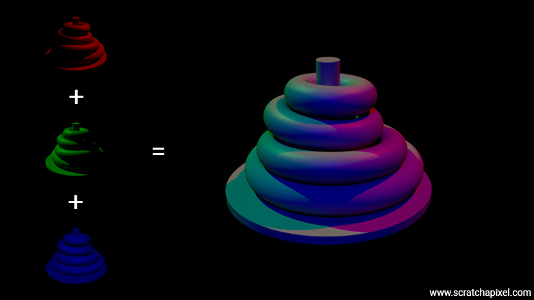
Another way to see this is by considering what you would be doing if you were to render a scene with three lights. You could render one image per light and then add these images together in compositing software (check the figure below). This would have the same effect as rendering the scene with the three lights and summing their contributions in the light loop.

Do not mix the light loop with the loop over the light samples. In this particular lesson, and for simplicity's sake, we've been calculating shadows by generating multiple light sample directions per light. Where the number of light samples for any particular area light in this example is hard-coded (512 in the code snippet above). In most modern production renderers, this is not the most commonly chosen approach. The common approach consists of casting one light sample ray per light but calling the Li method multiple times per pixel. This means we have multiple samples per pixel instead of multiple light samples per light. By averaging the contributions over many pixel samples, we achieve the same result as if we had cast many light samples with a single call to Li. However, the former approach (calling the Li method multiple times per pixel) has other benefits that we will explain in the forthcoming lessons on the rendering equation and sampling strategies.

So again, for the time being and until we introduce the concept of pixel samples, let's just be happy with computing the shadows for our area light by casting several light samples per area light and averaging their contributions.

Many Lights Optimization: Hello to Importance Sampling

To conclude, we want to touch on a method we won't be studying the implementation of in this lesson, as it would take us too far for what remains an introduction to the topic. Furthermore, while we have introduced some concepts related to the Monte Carlo integration method in this lesson, the following technique, while again somehow relying on the same principles as Monte Carlo integration, is based on knowledge we haven't yet covered. So, we will just mention its existence here and consider studying it in detail either in a future revision of this lesson or in part 2, depending on which way we decide to go.

The issue with using area lights, as we mentioned before, is that even though computers have become fast enough for ray tracing, it remains expensive regardless. This wouldn't be much of a problem if people making CG images for a living, like those working in studios such as Pixar, didn't feel the need to render scenes with not just a handful but sometimes thousands of such lights. One of the scenes in the Pixar movie Coco has about 29,000 lights.

While it would be relatively easy to adjust our code to replicate this, I won't even dare to waste time going down that path. No point. The point is, we need to optimize further as scenes may contain many (many) lights. This is even more relevant when you consider that only a few of these 29,000 lights may contribute significantly to the brightness of a pixel. Those that are very bright but super far away, or those very large but not very bright, or those that have all possible imaginable weaknesses—being small and far away—would be wasteful to compute because they'd effectively contribute little to the brightness of a point. Now, from a statistical or mathematical standpoint, it's not because lights contribute little that they should be ignored entirely. In fact, if you were doing so, you'd be introducing what we call a bias. The bottom line is, they may individually contribute little, but if you have thousands of lights that add a small fraction of light to the scene, all together they may contribute a significant part of the scene's global illumination. Yep.

So what shall we do? Again, without going into much detail here, the general idea is to resort to the statistical nature of the Monte Carlo method, where you sample the lights and divide the result of evaluating each light by the probability of choosing that light versus the other lights. The idea behind dividing the result of evaluating the light contribution by the probability (PDF) of choosing this light is similar to why we divide the light contribution when using Monte Carlo sampling for choosing a light sample direction, by the PDF associated with sampling the shape of the light. It is necessary to ensure that the weight assigned to the chosen sample direction or light compensates for all the other directions or lights you haven't chosen, and that statistically, the result converges to the same result you would obtain if you were to sample all the directions or all the lights.

Think of it this way: if you decide that you will somehow preferably sample lights in the scene that have great power, then the PDF associated with sampling such lights will be greater. Meaning (since this is your goal) that you will be more likely to sample lights with great power than those with a power whose value is considered small. Imagine the PDF associated with sampling such light is 0.8. You evaluate one of these lights and divide its contribution by 0.8. Imagine the PDF associated with sampling low-power lights is 0.2 (the probability of sampling such lights is lower than the probability of sampling lights with large power values). Sometimes, but less frequently than bright lights, you will sample a dim light. But that's okay because you will divide its contribution by 0.2, effectively multiplying its contribution by 5, which compensates for all the other dimmer lights you haven't sampled as a result of them being less represented due to your chosen PDF. All things being equal (sampling all the lights or sampling some of the lights but dividing their contribution with the probabiliy of sampling those), in the end, you get the same result as if you had sampled all the lights (but you get a result much faster). Of course, as with every Monte Carlo integration method, this will introduce variance to your result, which appears as noise in the image (in addition to the noise you got from sampling the shape of the area lights). But that is the tradeoff. You cut down on your render time while staying at least statistically true to what the result would be if you had infinite computing power, at the expense of introducing noise into your image. We all know that nothing's perfect.

Different strategies exist for choosing a PDF that works for the multi-light sampling requirement. The most basic one consists of simply considering every light equal and coming up with a PDF equal to \(1 / Nl\) where \(Nl\) represents the number of lights in the scene. While not necessarily the best (this method would produce high variance), as you can guess, it's still valid and helps you already reduce the number of lights being used while still providing a result that would converge (over many runs) towards the ground truth result. Smarter strategies consist of sampling the lights based on their contribution (so proportional to their contribution), a technique known as importance sampling (you give importance to lights that contribute the most while at least from a statistically standpoint, still considering those that contribute less but compensating their less frequently sampled probability by multiplying their contribution with a larger weight).

This technique is common in shading and will also be used when it comes to materials, shaders, and BRDFs, which we will address in the following lessons.

Things that We Are Left to Study

As mentioned in the introduction of this lesson, we've left some topics aside to keep this lesson reasonably short and to allow us to move on to the next important lessons as quickly as possible. Most of the topics related to lights that are left untouched are not necessarily as important as those contained in the first version of this lesson. Topics that come to mind include:

• Disk area light shape.

• Projected cone angle sampling, which we touched on at the end of the previous chapter.

• Mesh lights.

• Multiple importance sampling in a scene containing many lights.

Rest assured that we will look into these topics either in a future revision of this lesson or in a part 2. Other light-related topics, such as environment lights and image-based lighting, will have their own dedicated lessons.