Introduction to Lighting

Triangular Area Light

Preamble

Because each shape that an area light can have has its own specific implementation considerations, we have decided to dedicate one page per area light shape. More specifically, we will consider triangular, planar, disk, and finally spherical area lights. This preamble is repeated on each page to ensure that if you landed on one of these pages from an external link, you are aware that it is advisable to start by reading the page on the triangular area light. There, we will discuss some concepts that will be reused across the other light types and provide a general explanation about the code we will be using to implement these lights.

Also note that we strongly recommend that you read the lessons on Distributed Ray-Tracing and Stochastic Sampling and Sampling Strategies, which are corollaries to this one.

The Triangular Area Light

We have decided to start the section devoted to the practical implementation of these area lights with the triangular area light type. Because we have already spent some time working with rectangular area lights in the previous chapter, we thought it would be insightful to explore how what we have learned in the more theoretical introduction to area lights applies to a light with a different shape. We hope this makes it a bit more interesting for you. The implementation for rectangular area lights will follow.

It's entirely possible to have an area light that takes the shape of a single triangle. Note by the way that a rectangular area light can be composed of two triangles. Also, if we know how to use a triangle as an area light, then a triangular mesh could also serve as an area light, since all we would need to do is apply what we will learn in this chapter to the individual triangles making up the mesh. However, we will leave this to future versions of this lesson.

Similarly to what we have learned in the previous chapter, we will be using the area sampling method for the triangle. In essence, what we will do is as follows:

• Choose a point on the surface of the triangle that is uniformly distributed across the surface. Uniform distribution means, as explained in the previous chapter, that every point we choose on the triangle has an equal probability of being picked as any other point.

• Since we chose a uniform distribution, we also know from the previous chapter that the probability distribution associated with this sampling method will be 1 over the triangle's area.

• Once we have the PDF and the point, we can calculate the light sample direction, \(\omega_i\), and also calculate the distance \(r\) from the shading point \(x\) to the sample \(x'\) on the triangle surface, which as also explained earlier in the lesson, is required by the inverse square falloff (which is part of the area sampling method).

• Repeat the points above, sum up the contributions of each sample, and ultimately divide the total by the number of samples used.

The image below show the 16 samples chosen by our program for a given shaded point. Now before we go any further note that until we reach the end of this chapter, we will ignore shadows.

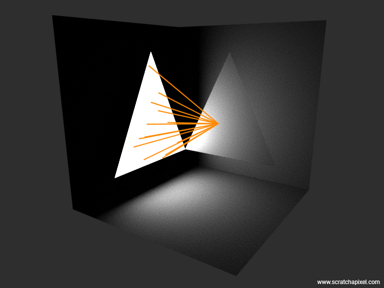
Remember that the equation we will be using is:

The first thing we need to do from an implementation standpoint is learn how to uniformly sample a triangle.

Uniformly Sampling a Triangle

Although sampling a triangle is not too complicated, it is also not as straightforward as sampling a rectangle. Most books do not clearly explain what we are trying to achieve here, especially in a way that is meaningful and clear. As usual, Scratchapixel will come to the rescue here and address this problem (perhaps it's time to consider a small donation?).

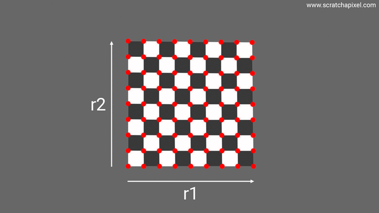
We have random number generators that can produce numbers that are independently and identically distributed (uniformly, in our case) across the range [0, 1]. In some texts, you will see this described as i.i.d. (independent and identically distributed) random variables, mathematically represented as \( X \sim U(0,1) \). Typically, we generate samples on a simple 2D surface such as a square or rectangle. Why 2D? Because there is a property in geometry known as affine invariance. It states that if a geometric property holds true for one shape (a square or a triangle), such as a unit square (with coordinates (0,0)-(1,1) for the lower-left and upper-right corners respectively) or the "unit" triangle (defined by the coordinates (0,0), (1,0), (1,1)), then it must hold for every other quadrilateral or triangle, since we can find an affine transformation between them. Remember, an affine transformation is one that preserves points, straight lines, and planes. Specifically, it preserves ratios of segments and mean points by linearity.

This rule is important, because generating a sample on the surface of the 2D unit square is simpler than generating one on a generic quadrilateral, as we will show in a moment. Once you have your sample on the 2D unit square or your "canonical" triangle, you can apply the same technique to sample any other quadrilateral or triangle thanks to the affine invariance property, including 3D ones, since a 2D unit square or triangle is essentially a 3D triangle lying in a plane. Number 1 problem explained.

Then, why is the unit square cool? Because we can sample the unit square by just generating two such i.i.d. random numbers with a uniform distribution: the first random number gives you the sample's x-coordinate, while the second gives you the y-coordinate. Great. But for the sake of this chapter, what we need is not a point in a square but a sample in a triangle. So the challenge is to map the two random numbers that we used to sample the unit square into a triangle. Most, if not all, the science of sampling shapes consists (well, most of the time at least) of finding how to map some random numbers generated on the unit square into some other fancy shape, be it a disk, a triangle, etc. It is a mapping process. And the key to this mapping is to preserve the distribution that you used to sample a point on the unit square (our two random numbers) while mapping the sample to its final shape, say the triangle in our present case. And this is where things can get tricky, as we will see with some mapping methods later.

The next animation illustrates this idea, where you can see a square morphing into a triangle. Note how the samples, which for the sake of demonstration are neatly snapped at regular intervals, are pushed to a new location as the square morphs into a triangle. So again, the problem we want to solve here is: What sort of transformation process or equation, if you will, will map a sample with a uniform distribution—whose coordinates are obtained by generating two random numbers in the range [0, 1] with a uniform distribution—over the unit square into the triangle, so that the uniform distribution of samples on the square is also uniform when mapped onto the triangle? Problem number 2 explained.

Note one extremely critical thing that this animation helps visualize, which is that we have the same number of samples in the final triangle as in the initial square. And yet, the triangle is half the area of the unit square. What does that imply? That the density of samples on the triangle is twice that of the square. This is a super key observation because remember that the area of a square-rectangle is \(xy\) where \(x\) and \(y\) define the rectangle's dimensions. Ok, here we deal with a square, but the idea is the same and it doesn't hurt to generalize. As explained in the previous chapter, the PDF or probability density function of a rectangle is the rectangle's area. Indeed, if we want to uniformly distribute samples across the surface of a rectangle, it makes sense to think that each sample, on average, covers an equal small area of the rectangle, the sum of which being the area of the rectangle itself. So the probability density of the rectangle is indeed \(xy\). And so, if the density of samples is twice as high for the triangle, the triangle's probability density is \(2xy\). This will become handy for some of our later demonstrations, so keep this in mind.

Note also that when you "morph" the unit square into your triangle, the property we are trying to preserve is the area (of the sample). This means if the samples have a uniform distribution on the unit square and assuming the mapping preserves this uniform distribution once mapped into the triangle, the samples within the triangle should also have equal areas. This is known as an area-preserving transformation. The areas of individual samples don't have to be the same (we have shown that the density of samples doubles when mapped onto the triangle, so clearly the area of any individual sample is half that of the equivalent sample on the unit square), but the scale factor must be constant for all samples after transformation. In mathematics, this concept is captured by the term Jacobian, which you are likely to see in textbooks and forums like Stack Overflow where mathematicians are answering your questions. The transformation is defined by a matrix, and the Jacobian of this matrix refers to the determinant of the matrix, which indicates the factor by which area elements are scaled by the transformation at a point. For an area-preserving transformation, the Jacobian determinant should be constant (the same everywhere), indicating that the transformation has preserved the area property. The Jacobian term, explained at last.

That ends the part that no one ever tells you about. Now that you are as well-equipped as any engineer, let's explore some methods for accomplishing this. Some methods may fail (intentionally, so you understand why books dedicated to this topic exist—it's not as trivial as it may seem), and some will succeed.

Mapping the unit square to the unit triangle: The (Failing) Naive Method

For the sake of the demonstration, we will work on a 2D triangle whose origin (first vertext is a the origin). Here is the code for this method:

Vec2f NaiveMethod(const Vec2f& v1, const Vec2f& v2, float r1, float r2) {
	return /* (1 - r1) * v0 + */ r1 * (1 - r2) * v1 + r1 * r2 * v2;
}

template<typename  SamplingMethod>
void SampleTriangle(SamplingMethod sample) {
	std::random_device rd;
	std::mt19937 eng(rd());
	std::uniform_real_distribution<float> distr(0.f, 1.f);
	for (size_t i = 0; i < nsamples; ++i) {
		// We assume v0 = (0,0)
		sample({2,0}, {1,2}, distr(eng), distr(eng));
		// plot x...
	}
}

Note that to generate random numbers uniformly distributed, we simply use the random number generators from the C++ standard library. If you are interested in understanding how it works, we move the sample along the v0v1 edge using u, which is a uniformly distributed random number in the range [0, 1]. The term (1.f - u) adjusts the influence of v2 based on how far along the edge from v0 to v1 the point has moved: the further along, the less influence v2 should have. The v further scales this influence.

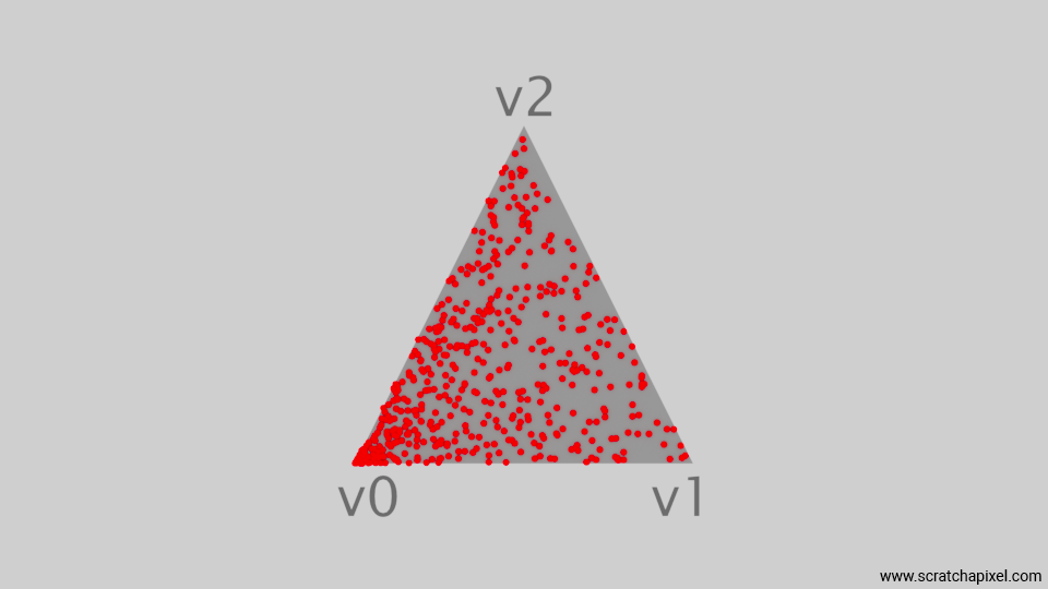
The "naive" method does not work effectively. It’s enough to look at the image below, showing the results, to notice a concentration of samples near one of the triangle's vertices. Clearly, this method fails to distribute the samples uniformly across the surface of the triangle. We will explain why this method is ineffective when we discuss the square-root optimization method.

The Uniform Distribution Trilinear Coordinates Picking Method (Fails Too)

Another idea would be to pick the barycentric coordinates of the triangle from a uniform distribution as follows:

Vec2f BarycentricCoordinatesMethodBad(const Vec2f& v1, const Vec2f& v2, float u, float v, float w) {
	float sum = u + v + w; // we need to normalize the barycentric coordinates
	return /* (u / sum) * v0 + */ (v / sum) * v1 + (w / sum) * v2;
}

template<typename SamplingMethod>
void SampleTriangle(SamplingMethod sample) {
    std::random_device rd;
    std::mt19937 eng(rd());
    std::uniform_real_distribution<float> distr(0.f, 1.f);
    for (size_t i = 0; i < nsamples; ++i) {
		// We assume v0 = (0,0)
        Vec2f x = sample({2, 0}, {1, 2}, distr(eng), distr(eng), distr(eng));
        // plot x...
    }
}

Remember that barycentric coordinates can help us define any point on the triangle, but the sum of these coordinates is required to be 1. We can generate three random numbers in the range 0 to 1, sum them up, and divide them by this sum to normalize them. We can then simply use these coordinates to calculate the position of a sample on the triangle. Note that since in our example, we assume that v0 is at the origin, we can skip u. Here is the result:

As you can now see, the samples are pushed towards the center of the triangle. This does not result in a uniform distribution either. Showing these incorrect methods might not seem particularly interesting or valuable, but it serves to emphasize, as we will frequently observe with subsequent shapes, that uniformly sampling a triangle is not as straightforward as it might appear. Hopefully, we can still make this method work with some adjustments. This method is known as the Square-Root optimization method which also relies on the use of barycentric coordinates.

The (Winning) Square-Root Optimization Method

I will provide the equation and explain why this method works (because this one does). The equations to uniformly sample a triangle using barycentric coordinates using the square-root optimization method are:

where \(\varepsilon_1\) and \(\varepsilon_2\) (or r1 and r2 in the code) are two independent and identically distributed random variables. Note that we are using \(X\) and \(Y\) in place of u and v to conform with the notation most commonly seen in discussions on this topic. Since we are constructing \(X\) and \(Y\) from \(\varepsilon_1\) and \(\varepsilon_2\), which are random variables, \(X\) and \(Y\) are random variables themselves. However, they are not independent of each other because both depend on \(\varepsilon_1\) and \(\varepsilon_2\). With that, we can see that \(0 \leq X, Y \leq 1\) and \(X + Y \leq \sqrt{r_1} \leq 1\). The first statement is obvious since both \(\varepsilon_1\) and \(\varepsilon_2\) are in the range [0, 1]. As for the second statement:

These equations are crucial to demonstrate that the point is always within the triangle. We now need to prove that this point is also evenly distributed across the triangle. This technique was initially introduced by Greg Turk in the book *Graphics Gems* (1990, p. 24). The issue with Greg's initial presentation is that it doesn't provide a formal explanation as to why the resulting distribution is uniform. Instead, his explanation is informal but can help us gain an intuition as to why this works before we delve into the complex mathematics of it.

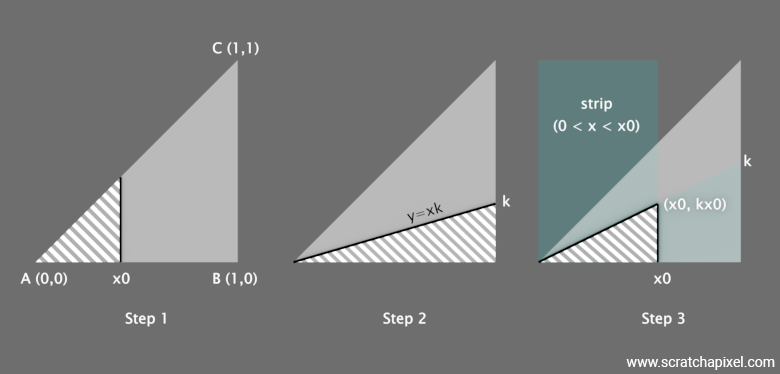
As previously mentioned, when mapping from the unit square to the triangular shape, it's essential that this mapping preserves the area. Below, you will find a triangle with vertices \(A = (0,0)\), \(B = (0,1)\), and \(C = (1,1)\). This triangle can be visualized as a unit square with its top-right vertex shifted to the top-left. We have relabeled the x- and y-coordinates to s- and t-coordinates, following the notation used by Turk.

Imagine drawing a line every 0.1 unit along the t-axis from 0 to 1, parallel to the s-axis. This divides the triangle into 10 sections. Now, envision filling each section with 4 balls. Consider how these balls would appear on the unit square before the top-right vertex is moved to the top-left. In the unit square, the 4 balls in the top row—originally a rectangle—would be compressed into a smaller triangular area at the top, unlike the balls in the bottom row, which would occupy a rectangular area with a slanted right edge. In the unit square, the 4 balls in each row are evenly distributed, which represents a uniform distribution.

However, in the triangular configuration (the illustration should clarify that), the balls are not evenly distributed; they occupy areas of varying sizes. The uniform distribution property is no longer preserved.

In conclusion, if we were to generate points by randomly selecting uniform floating numbers from [0,1] and distributing these along the s-axis using another random number, there would be a higher concentration of points near the vertex \(A\) than at the base. This is because the closer you are to \(A\), the more densely packed the samples become. This illustrates why a naive approach fails, resulting in an increased sample density near \(A\).

This is where the square root of \(t\) becomes crucial. In the figure's top-right triangle, we've now spaced the lines using \(\sqrt{t}\) rather than \(t\), with \(t\) still increasing in increments of 0.1 units. Specifically, the spacing is \(\sqrt{0.1}, \sqrt{0.2}, \sqrt{0.3}, \ldots, \sqrt{0.9}\). You'll notice the lines are no longer equidistant, reflecting the characteristics of the square root function. Looking at the plot of the square root function (bottom-left), you can see that the values for \(y\) increase more rapidly when \(x\) is less than 0.5 and then level off to resemble more of a straight line. If you were to calculate the area of each region defined by these lines, you would find they are now all equal, each with a value of 0.05 in this specific setup.

What does this mean for those of us who aren't mathematicians? It implies that if you distribute points using the square root of a random number for \(t\) and another random number for \(s\), you'll achieve a uniform distribution of samples across the triangle's surface. This effect comes from stretching the triangle’s "density" so that, for example, the four balls in the first row occupy the same space as the four balls in the last row.

That's the intuition provided by Turk (though the book distills this into a single line). If you're looking for a more formal proof, check the box below—but feel free to skip it if you're not deeply into mathematics.

First, let's give credit where credit is due. The following answer is a rewrite of the very elegant solution provided on Math StackExchange. I have derived all the steps to ensure you fully understand the answer, which is very compact. The thread also proposes another solution, which demonstrates that the probability of being within an area \((0,x) \times (0,y)\) is \(2xy\) through integration (I explained in the introduction of this chapter why the probability is \(2xy\) and why that is twice the probability of the square though). However, this requires more work than the first solution. For now, I have only chosen to present the first one. Follow the link to explore the second method as well if you want to.

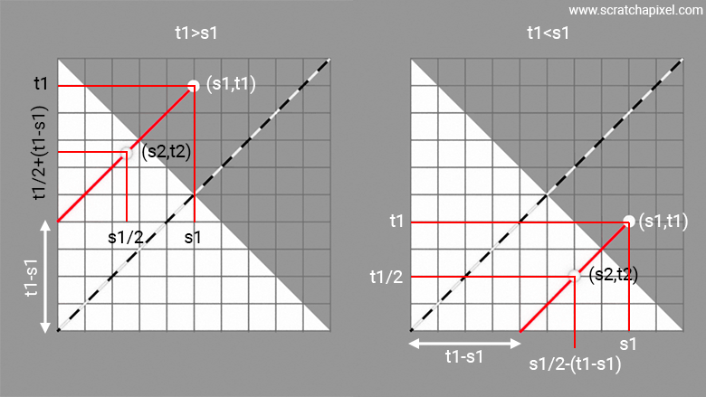
There are a couple of ways by which we can prove that the coordinates \((\sqrt{r_1}, \sqrt{r_1} r_2)\) lead to a uniform distribution on a triangle. Consider a triangle formed by the vertices \(A, B, C = (0,0), (1,0), (1,1)\). We can say that a point \((x,y)\) is in the triangle if \(0 < x < 1\) and \(0 < {y}/{x} < 1\). You can easily verify the second condition by looking at an image below, where you can check that any point within the triangle has an x-coordinate that is necessarily greater than or equal to (if we consider a point on the line \(BC\)) its y-coordinate, and thus the ratio \({y}/{x}\) is necessarily less than 1.

The proof involves examining the distributions of \(x\) and \({y}/{z}\) respectively. To understand the following explanation, it's crucial to recognize this one important property of uniform distribution:

By definition, a random variable \(X\) uniformly distributed over the interval [0,1] implies that every point within this interval is equally likely to occur. The probability that \(X\) falls within any subinterval is equal to the length of that subinterval. For example, if \(X\) is uniformly distributed between 0 and 1, the probability that \(X\) is less than 0.9 is 0.9. This reflects the uniform distribution where the likelihood of falling within any segment is proportional to its length. We'll refer to this as the uniform probability property.

Step 1 - Goal: show that \(x^2\) is uniformly distributed. The first thing we aim to prove is that for any point \(x_0\), \(P(0 < x < x_0) = x_0^2\) (where \(P(0 < x < x_0)\) is called a Cumulative Distribution Function, or CDF). This expression means that the probability that \(x\) is greater than 0 and less than \(x_0\) (where \(x_0\) ranges between 0 and 1) equals \(x_0^2\). If we select a point \(x_0\) on the x-axis, the point \((x_0, x_0)\) lies on the line \(y = x\), which is within the triangle since \(y \leq x\) for \(0 \leq x \leq 1\). The triangle formed by this point and the x-axis will have a base of \(x_0\) (from \(0\) to \(x_0\) on the x-axis) and a height of \(x_0\) (from the x-axis vertically up to the line \(y = x\)). The area of this triangle is calculated using the formula for the area of a triangle:

$$ \text{Area} = \frac{1}{2} \times \text{base} \times \text{height} = \frac{1}{2} \times x_0 \times x_0 = \frac{1}{2} x_0^2 $$

The area of the smaller triangle (where \(x \leq x_0\)) relative to the area of the larger triangle (the right triangle \(ABC\)) represents the probability that a randomly chosen point within the larger triangle has an \(x\)-coordinate less than \(x_0\). Since the larger triangle encompasses the entire region between \(x = 0\) and \(x = 1\), the total area of this triangle is also \({1}/{2}\) (half of the unit square). The probability \(P(0 < x < x_0)\) relates to the ratio of the smaller triangle's area to the whole triangle's area. If the total area were normalized to 1 (ignoring the \({1}/{2}\) scaling), then the area of the smaller triangle directly gives the cumulative probability for \(x\) being less than \(x_0\), which is \(x_0^2\).

If \(P(0 < x < x_0) = x_0^2\), then by setting \(x_0 = \sqrt{a}\), we get \(P(0 < x < \sqrt{a}) = (\sqrt{a})^2 = a\). This shows that the probability that \(x^2\) is less than any \(a\) in [0, 1] is \(a\), matching the characteristics of a uniform distribution (as per the definition above). The key insight here is that we have proven \(x^2\) to be uniformly distributed.

Step 2 - Goal : show that \(x/y\) is uniformly distributed: Then we need to check that \(P(0 < {y}/{x} < k) = k\). Similarly to the previous proof, we assume that \({x}/{y}\) is also uniformly distributed on [0,1]. We also have \(0 < x \leq 1\) and \(0 \leq y \leq x\). The ratio \({x}/{y}\) ranges from 0 to 1. We want to find the probability that the ratio \({x}/{y} \leq k\) with \(k\) being a number in the interval [0,1]. The condition \({x}/{y} \leq k\) can be visualized on the triangle. Draw a line from the origin (0,0) with a slope of \(k\) (i.e., \(y = kx\)). For \(k \leq 1\), this line will intersect the line \(x = 1\) at point (1,k). The area below this line and above the x-axis, within the triangle, represents the points satisfying \({y}/{x} \leq k\). The area below the line \(y = kx\) within the triangle can be calculated as a right triangle with base \(1\) and height \(k\). The area of this triangle is \({1}/{2} \times \text{base} \times \text{height} = {1}/{2} \times 1 \times k = {k}/{2}\).

The total area of triangle \(ABC\) is \({1}/{2}\) (as the triangle is right-angled and spans from \(0\) to \(1\) on both the x and y axes). The probability that \(\frac{y}{x} \leq k\) is the ratio of the area of the triangle below the line \(y = kx\) to the total area of the triangle \(ABC\):

$$ P\left(0 < \frac{y}{x} \leq k\right) = \frac{\text{Area below } y = kx}{\text{Total area of } ABC} = \frac{\frac{k}{2}}{\frac{1}{2}} = k $$

This shows that the cumulative distribution function \(P\left({y}/{x} \leq k\right) = k\), indicating that the ratio \({y}/{x}\) is uniformly distributed from 0 to 1 Remember the uniform distribution property here. If the ratio \( {x}/{y} \) mirrors the fundamental property of a uniformly distributed variable, then the likelihood of the variable being within any segment [0, k] of the distribution's range [0, 1] should be \(k\).

Step 3 - Goal: Show that \(x^2\) and \(x/y\) are independant: Finally, we need to prove that \(P(0 < x < x_0 \land 0 < {x}/{y} < k) = x_0^2k\). The expression \( P(0 < x < x_0 \land 0 < \frac{y}{x} < k) = x_0^2 k \) represents what we call a joint probability. I wan't delve too much here about this means, you can check the lesson on probality for that, but in short, it is the probability that both \( x \) falls within a specific interval \((0, x_0)\) and simultaneously, the ratio \( {y}/{x} \) falls within another interval \((0, k)\). The proof of this, which relies on an area computation again, will serve to demonstrate that \( x^2 \) and \( {y}/{x} \) are independent random variables.

We want to calculate the probability of two conditions being satisfied simultaneously within the triangle defined by points \((0,0), (1,0), (1,1)\):

$$ \begin{array} 0 < x < x_0 \\ 0 < \frac{y}{x} < k \end{array} $$

The triangle ABC where \(0 \leq x \leq 1\) and \(0 \leq y \leq x\) has an area of \( {1}/{2} \). The first condition \(0 < x < x_0\) confines the point to be within a vertical strip from \(x = 0\) to \(x = x_0\). The second condition \(0 < {y}/{x} < k\) implies that for each \( x \), \( y \) must be less than \( kx \) (see figure). Within the strip where \(0 < x < x_0\), the line \( y = kx \) defines a smaller triangle if \(k \leq 1\). The vertex of this smaller triangle is at \((x_0, kx_0)\), given that \(x_0 \leq 1\) and \(kx_0 \leq x_0\). The area of this sub-triangle is given by:

$$text{Area} = \frac{1}{2} \times \text{base} \times \text{height} = \frac{1}{2} \times x_0 \times kx_0 = \frac{1}{2} kx_0^2$$

Since we previously found that the total area of the triangle ABC (if normalized) relates the probabilities directly to the areas of sub-regions, and since the total triangle has area \( {1}/{2} \), the normalized probability is:

$$P(0 < x < x_0 \land 0 < \frac{y}{x} < k) = \frac{\frac{1}{2} kx_0^2}{\frac{1}{2}} = kx_0^2$$

From earlier, we know \(P(0 < x < x_0) = x_0^2\) and \(P(0 < {y}/{x} < k) = k\). If \(x^2\) and \( {y}/{x}\) were independent, the joint probability \(P(A \cap B)\) should equal \(P(A)P(B)\). Calculating it gives:

$$P(0 < x < x_0)P(0 < \frac{y}{x} < k) = x_0^2 \times k = kx_0^2$$

This is equal to the calculated joint probability, confirming that \(x^2\) and \({y}/{x}\) are independent, as their joint probability equals the product of their individual probabilities.

Conclusion: We have demonstrated that to generate a point uniformly within the triangle, one can select values for \(r_1\) and \(r_2\) uniformly from the unit interval [0,1], where \(x^2 = r_1\) and \(\frac{y}{x} = r_2\). From these, we calculate the coordinates \((x, y)\) as \((\sqrt{r_1}, r_2\sqrt{r_1})\). This method confirms that \(x^2\) and \(\frac{y}{x}\) are indeed uniformly distributed. The coordinates \((x, y)\) correspond to the barycentric combination of the triangle's vertices \(A\), \(B\), and \(C\), with respective weights \(1-\sqrt{r_1}\), \(\sqrt{r_1}(1-r_2)\), and \(\sqrt{r_1}r_2\). Thus, the point \((x,y)\) not only is uniformly distributed within the triangle but also illustrates the independence of \(x^2\) and \(\frac{y}{x}\), underpinning the uniform distribution of points within the triangle.

Now that we have shown that the equation provides a uniform distribution of points across the surface of the triangle, let's explore how this can be applied to our 3D triangle. So far, we have generated 2D samples in the triangle with coordinates (0,0), (1,0), (1,1), though we know that what works for this triangle will work for any other triangle, thanks to the affine invariance property. Next, we need to transform this 2D point into a 3D point. As pointed out in the introduction, we can assume that our 2D triangle is just a 3D triangle lying in a plane, so we are left with finding a method to convert the position of the 2D samples to barycentric coordinates, which applied to the vertices of the 3D triangle will give us to the position of the sample on the triangle but in 3D space.

Recall that the way we calculate a point \(P\) on a triangle using barycentric coordinates is as follows: \(\alpha A + \beta B + \gamma C\), where \(\alpha\), \(\beta\), and \(\gamma\) are the barycentric coordinates, \(A\), \(B\), and \(C\) are the triangle's vertices. We've already discussed barycentric coordinates at length in the lesson on Rasterization.

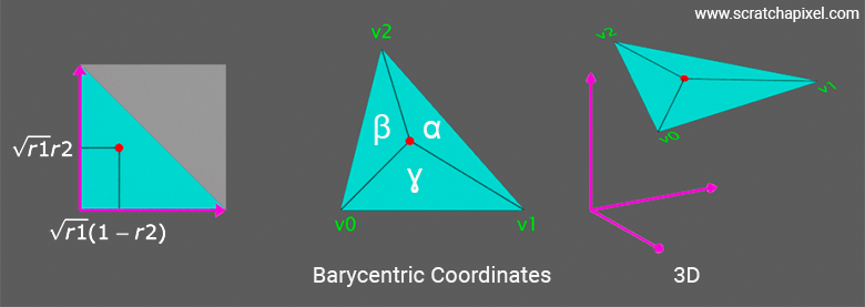
Note that, per the barycentric coordinate definition, \(\alpha + \beta + \gamma = 1\) (there are only two degrees of freedom). Thus we only need two of such coordinates to find the third one. Now, given a point \((x, y)\) in the unit triangle, we can express it as a combination of the unit triangle's vertices:

To map this point to an arbitrary triangle in 3D space using barycentric coordinates \((\alpha, \beta, \gamma)\):

With \(v0 = (0, 0)\), \(v1 = (1, 0)\), and \(v2 = (0, 1)\). And remember that going from \(P_{unit}\) to \(P_{3D}\) works thanks to the affine invariance property. In the coordinates given for \(v0\), \(v1\), and \(v2\), we haven't specified a z-coordinate, but remember that a 3D triangle can be seen as a 2D triangle lying in a plane. So the barycentric coordinates \((\alpha, \beta, \gamma)\) in the unit triangle are directly related to Cartesian coordinates:

The equation to calculate the point's position on the triangle is:

Here is the code to plot samples generated by this method:

Vec2f BarycentricCoordinatesMethodGood(const Vec2f& v1, const Vec2f& v2, float r1, float r2) {
	float q = std::sqrt(r1);
	// v0 = (0,0) so skip calculation
	return /* (1 - q) * v0 + */ q * (1 - r2) * v1 + q * r2 * v2;
}

template<typename  SamplingMethod>
void SampleTriangle(SamplingMethod sample) {
	std::random_device rd;
	std::mt19937 eng(rd());
	std::uniform_real_distribution<float> distr(0.f, 1.f);
	for (size_t i = 0; i < nsamples; ++i) {
		// We assume v0 = (0,0)
		Vec2f x = sample({2,0}, {1,2}, distr(eng), distr(eng));
		// plot x...
	}
}

int main() {
	SampleTriangle(BarycentricCoordinatesMethodGood);
};

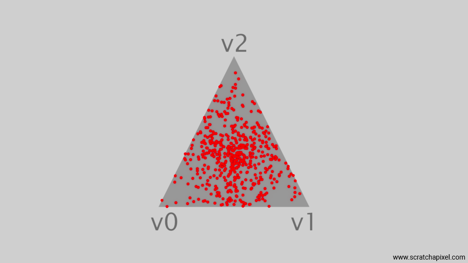
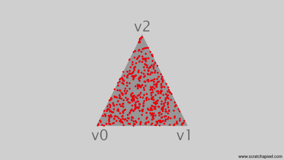
The next figure shows a plot of the resulting samples. As you can see, there is not a higher concentration of samples in any particular area of the triangle. While some clusters remain (a result of choosing random uniform numbers), the distribution is more uniform than what we have produced so far.

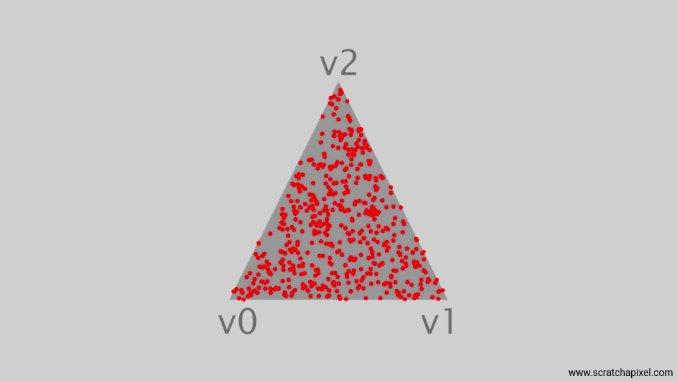
This is great, because this is effectively the technique we will be using to generate our samples on the triangular area light. While we could jump straight to that part, let's first mention a few more techniques to generate samples uniformly for the sake of completeness.

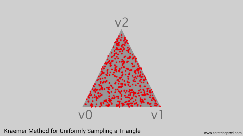
The (Alternative) Kraemer Method

The Kraemer method is quite interesting. The formal mathematical definition can be a bit cumbersome, so I will explain it within the context we need it for, which is the weighted average of the three points—the three vertices of our triangle. The idea is to generate two random numbers within the range [0, 1]. However, for the Kraemer method to work effectively, we need to ensure that \( \varepsilon_1 \), the first random number, is less than the second number \( \varepsilon_2 \). If this is not the case when we first generate them, we may have to switch their order. Once we have these two numbers sorted by increasing value, we calculate three coordinates (which you can see as a form of Barycentric coordinates), u, v, and w. The code is as follows:

Vec2f KraemerMethod(const Vec2f& v1, const Vec2f& v2, float r1, float r2) {
    if (r1 > r2) std::swap(r1, r2);
    float u = r1, v = r2 - r1, w = 1 - r2;
    return /* u * v0 + */ v * v1 + w * v2;
}

In this way, you can see u, v, and w representing the lengths of three segments whose sum is equal to 1 (as depicted in the figure below).

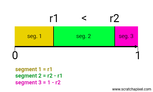
Summing the triangle vertices by these normalized coordinates provides us with a point uniformly distributed across the surface of the triangle.

Sorting out the random numbers can be avoided:

Vec2f KraemerMethod(const Vec2f& v1, const Vec2f& v2, float r1, float r2) {
    float q = std::abs(r1 - r2);
    float u = q, v = 0.5f * (r1 + r2 - q), w = 1 - 0.5 * (q + r1 + r2); // could more simply be w = 1 - u - v;
    return /* u * v0 + */ v * v1 + w * v2;
}

The (Alternative) Rejection Method and the Parallelogram Method

The rejection method is a classic approach to selecting random, uniformly distributed points. It's effective because it can be applied to virtually any shape. When used for our triangle problem, it involves continuously generating random points until a point that fits inside the triangle is found.

float r1, r2;
do {
	r1 = distr(gen);
	r2 = distr(gen);
} while (r1 + r2 > 1);
// r1 and r2 are now within the triangle. Use these coordinates for sampling.
...

This method may not be directly related to the problem at hand, but it's worth knowing about as you might encounter it in other contexts where it can be quite useful. Another method, known as the parallelogram method, involves generating a sample using two random floating points uniformly distributed in the range [0,1]. If the point is inside the triangle, it is used as is; if not, we simply reflect the point about the center of the parallelogram.

Vec2f RejectionMethod(const Vec2f& v1, const Vec2f& v2, float r1, float r2) {
	if (r1 + r2 > 1) {
		r1 = 1 - r1;
		r2 = 1 - r2;
	}
	return /* (1 - r1 - r2) * v0 + */ r1 * v1 + r2 * v2;
}

The (Alternative and Potentially Better) Low-Map Distortion Method

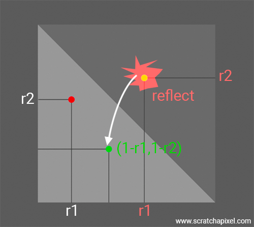
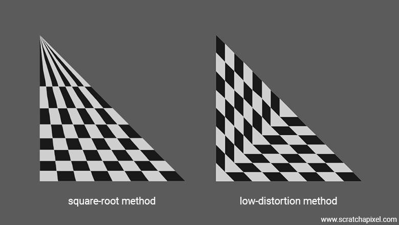
Eric Heitz proposed a method for mapping samples from the unit square to a triangle in his 2019 paper titled "A Low-Distortion Map Between Triangle and Square." This method is simple, fast, and avoids the main issues associated with the square-root optimization method, which stretches the mapping space to preserve uniform distribution, resulting in undesirable distortion.

The GIF animation at the beginning of the chapter, where you can see a square morphing into a cube, actually depicts the mapping technique proposed by Eric Heitz. It involves shifting each point on the unit square along a line parallel to the diagonal from point (0,0) to (1,1). The shift is half the distance between the edge of the square and the point to be remapped, as shown in the image below. With simple mathematics, one can easily calculate the new sample position on the triangle. You just need to determine the equation of the line parallel to the diagonal, which is \((t-s) + x\) where \((s,t)\) are the coordinates of the sample point in the unit square (output of two randomly uniformly distributed numbers). Consider two cases:

• When \(t > s\): the sample on the unit square is outside our triangle. Then, by construction (with \((s',t')\) being the positions of the remapped sample on the triangle):

  $$ \begin{array}{rl} s' = \frac{s}{2}, \\ t' = (t-s) + s' = (t-s) + \frac{s}{2}, \\ t' = t - \frac{s}{2} \end{array} $$

• When \(t < s\):

  $$ \begin{array}{rl} t' = \frac{t}{2}, \\ s' = t' - (t-s) = \frac{t}{2} - (t-s), \\ s' = s - \frac{t}{2} \end{array} $$

In code, this translates to:

Vec2f LowDistortionMethod(const Vec2f& v1, const Vec2f& v2, float r1, float r2) {
	if (r2 > r1) {
		r1 *= 0.5f;
		r2 -= r1;
	} else {
		r2 *= 0.5f ;
		r1 -= r2;
	}
	return /* (1 - r1 - r2) * v0 + */ r1 * v1 + r2 * v2;
}

This method efficiently maps the points, maintaining a more accurate representation within the triangular area, reducing distortion significantly.

The Pros and Cons of Each Method

In practice, all rendering engines we've examined employ the square-root optimization method, with variations in their implementation but similar outcomes. This method is particularly effective when extending the algorithm to higher dimensions. Another important consideration involves the use of low-discrepancy sequences (LDSs), or quasi-random numbers. These numbers are superior to purely random ones because they spread more evenly over the domain of interest, such as the range [0:1], while still retaining randomness. However, the use of quasi-random number generators can disrupt some properties of the low-discrepancy sequences when the parallelogram method is applied, which is undesirable. Therefore, it's advisable to avoid this combination. While this is a topic for a more advanced lesson, sticking to the square-root optimization method or avoiding quasi-random sequences generally ensures satisfactory results.

To conclude, the Low-Distortion Map method proposed by Eric Heitz has proven to run faster (20% faster in their GPU implementation) and is potentially free of the distortion commonly associated with the square-root optimization method. Therefore, this method should ideally be used.

Implementation: Putting It All Together

Now that we have a method for generating the samples across the surface of the triangle, we've assembled nearly all the elements necessary to implement a triangle area light. Our code will utilize the framework outlined in the lesson Core Components to Build a Ray-Tracing Engine from Scratch: A DIY Guide.

Firstly, we will add a triangular light to our scene:

std::shared_ptr<TriangleLight> light = std::make_shared<TriangleLight>(
    Vec3f(-1, -1, 0), 
    Vec3f(1, -1, 0), 
    Vec3f(0, 1, 0), 
    Vec3f(5.f));

Matrix44<float> xfm_light(0, 0, -1, 0, 0, 1, 0, 0, 1, 0, 0, 0, -1, 0, -4, 1);
prims.push_back(std::make_unique<Primitive>(light, xfm_light));

The triangular light will be implemented as a class derived from the AreaLight class.

class TriangleLight : public AreaLight {
public:
    TriangleLight(const Vec3f& v0, const Vec3f& v1, const Vec3f& v2, const Vec3f& Le)
        : v0_(v0), v1_(v1), v2_(v2), e1_(v1 - v0), e2_(v2 - v0), Ng_(e1_.Cross(e2_)), Le_(Le),
          tri_(new Triangle(v0, v1, v2)) {}

    std::shared_ptr<Light> Transform(const Matrix44f& xfm) const override {
        Vec3f v0, v1, v2;
        xfm.MultVecMatrix(v0_, v0);
        xfm.MultVecMatrix(v1_, v1);
        xfm.MultVecMatrix(v2_, v2);
        return std::make_shared<TriangleLight>(v0, v1, v2, Le_);
    }

    std::shared_ptr<Shape> GetShape() override { return tri_; }

    Vec3f Sample(const DifferentialGeometry& dg, Sample3f& wi, float &tmax, const Vec2f& sample, bool debug) const override {
        ...
    }
	
	Vec3f Le() const override { 
		return Le_; 
	}

private:
    Vec3f v0_;
    Vec3f v1_;
    Vec3f v2_;
    Vec3f e1_;
    Vec3f e2_;
    Vec3f Ng_;
    Vec3f Le_;
    stda::shared_ptr<Triangle> tri_;
};

I have left the Sample method incomplete as we will delve into it later. For now, just note how the triangular area light is constructed. The constructor takes three vertices that define the shape of the light in object space (its default shape). When building the scene, we call the Transform method to obtain the triangle transformed by its transformation matrix (other than the identity matrix, if specified). This transforms the shape of the triangle to world space. Note that while implementations may vary from engine to engine, in general, you want to see the area light in your image. Therefore, most implementations tend to associate a mesh with the light. In this case, when we construct the triangle area light, the instance of the light will also build an instance of Triangle, which is nothing but a Shape (a renderable geometry). Here is the implementation of the Triangle class:

class Triangle : public Shape {
public:
    Triangle(const Vec3f& v0, const Vec3f& v1, const Vec3f& v2)
        : v0_(v0), v1_(v1), v2_(v2), Ng_((v1 - v0).Cross(v2 - v0).Normalize()) {}

    std::shared_ptr<Shape> Transform(const Matrix44<float>& m) const override {
        Vec3f v0, v1, v2;
        m.MultVecMatrix(v0_, v0);
        m.MultVecMatrix(v1_, v1);
        m.MultVecMatrix(v2_, v2);
        return stda::make_shared<Triangle>(v0, v1, v2);
    }

    size_t GetNumTriangles() const override { return 1; }
    size_t GetNumVertices() const override { return 3; }
    Box3f Extract(size_t id, BuildTriangle* triangles, size_t& num_triangles, Vec3f* vertices, size_t& num_vertices) const override {
        Box3f bounds;
        triangles[num_triangles++] = {(int)(num_vertices), (int)(num_vertices + 1), (int)(num_vertices + 2), (int)id};
        vertices[num_vertices++] = v0_;
        vertices[num_vertices++] = v1_;
        vertices[num_vertices++] = v2_;
        bounds.ExtendBy(v0_);
        bounds.ExtendBy(v1_);
        bounds.ExtendBy(v2_);
        return bounds;
    }

    void PostIntersect(const Ray& ray, DifferentialGeometry& dg) const override {
        dg.P = ray.orig + dg.t * ray.dir;
        dg.Ng = Ng_;
        dg.Ns = Ng_;
        dg.st = Vec2f(dg.u, dg.v);
        dg.error = stda::max(std::abs(dg.t), dg.P.Max());
    }

    Vec3f v0_;
    Vec3f v1_;
    Vec3f v2_;
    Vec3f Ng_;
};

The triangle geometry making up the area light will be rendered alongside all other meshes in the scene. Here is how this is done and the magic for adding our triangular area light contribution. Keep in mind that we focus on direct lighting in this lesson. The Li() method of the Integrator class is called on every primary ray shot for every single pixel composing the image. Its role is to:

• Determine whether the primary ray hits any geometry in the scene (including potentially the geometry making up an area light).

• If it doesn't hit anything, return the background color.

• If it does hit something, calculate the intersection point's color by considering the intersected point's material and the lights in the scene. Keep in mind that for the time being, we will assume our surfaces are purely diffuse (or matte, as you prefer).

Within our framework, it is crucial to call the scene's PostIntersect method after each intersection. This method triggers the PostIntersect method of the intersected shape. These processes are critical for setting necessary variables to shade the intersection point, such as the normal and position, as explained in the lesson Core Components to Build a Ray-Tracing Engine from Scratch: A DIY Guide.

Vec3f Li(const Ray& ray, const std::unique_ptr<Scene>& scene) {
    const BuildTriangle* tris = scene->triangles_.get();
    const Vec3f* vertices = scene->vertices_.get();
    DifferentialGeometry dg;
    for (size_t i = 0; i < scene->num_triangles_; ++i) {
        Intersect(ray, dg, tris[i], vertices); 
    }

    scene->PostIntersect(ray, dg);

    // No intersection, return the background color (here middle grey).
    if (!dg) {
        return Vec3f(0.18);
    }
    
    // Calculate direct lighting (light loop)
    ...
    
    return L;
}

Now let's examine the light loop itself, where we will accumulate the contribution of each light to the brightness of the shaded point \(x\). This accounts for direct lighting only.

Vec3f Li(const Ray& ray, const std::unique_ptr<Scene>& scene, bool debug = false) {
	...
	Vec3f L = 0;

	if (dg.light)
		L += dg.light->Le();

	size_t num_samples = 16;
	for (size_t i = 0; i < scene->lights_.size(); ++i) {
		Vec3f L_light = 0;
		for (size_t n = 0; n < num_samples; ++n) {
			LightSample ls;
			ls.L = scene->lights_[i]->Sample(dg, ls.wi, ls.tmax, distr(eng), distr(eng));
			if (ls.L == 0 || ls.wi.pdf == 0 || dg.Ng.Dot(Vec3f(ls.wi)) <= 0.f) continue;
			L_light += 1 / M_PI * ls.L * dg.Ng.Dot(Vec3f(ls.wi)) / ls.wi.pdf;
		}
		L += L_light / num_samples;
	}

	return L;
}

First, if the object that intersected the primary ray is a triangular light, we add its contribution (dg.light->Le()) to the primary ray's returned color L (which we initialize to 0). Then, for each light in the scene (outer loop), we will loop over a given number of samples (inner loop), 16 in this code above. For each sample, we call the Sample() method of the current light, which is where we will select the position of a sample on the light surface from which we will be able to calculate the light sample direction wi. To calculate this sample position, we need two random numbers, which for now will be generated from a simple random number generator provided by the C++ standard library. You should know that there are much better ways of generating these numbers than just random numbers, but for our naive, first brute-force approach, we will work with a uniformly distributed random generator. Check the lesson Sampling Strategies to learn about the topic of generating better sequences of such numbers.

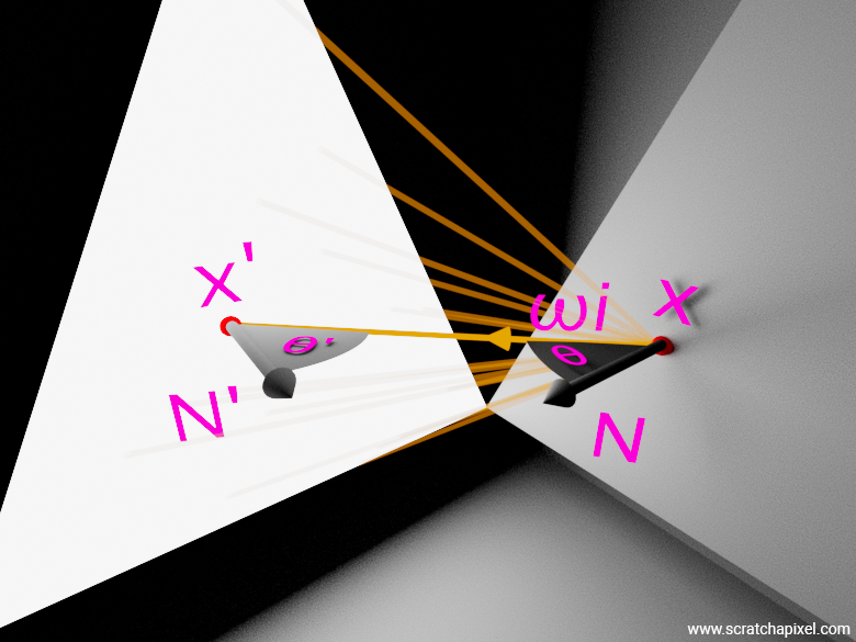
tmax is the distance from the shaded point \(x\) to the sample position \(x'\) as shown in the next figure. It will be used to limit the extent of the shadow ray. Note the use of the LightSample structure here:

template<typename T> 
struct Sample {
	operator const T&() const { return value; }
	operator T&() { return value; }
	T value;
	float pdf;
};

using Sample3f = Sample<Vec3f>

struct LightSample {
	Sample3f wi;
	float tmax;
	Vec3f L;
};

It holds the data for tmax and LightSample::L, the light radiant exitant value, in addition to an instance of type Sample3f, which is a structure that itself holds the sample direction \(\omega_i\) stored in value in the code above, and the pdf (stored in the pdf variable). We will see how these variables are set when we get to the code of the light Sample method. Note that before we add the contribution of the sample to L_light, the current light contribution, we check whether we effectively need to add the sample contribution by checking if either one of these conditions is true:

• Is the light radiant exitant LightSample::L greater than 0?

• Is the sample pdf greater than 0? If not, the sample doesn't contribute.

• Is the surface normal and the light sample direction pointing in opposite directions (the dot product of the two vectors would then be less than 0)? If this is true, then the surface would point away from the light, and the light would not contribute to the shaded point's illumination. Note that by construction, the light sampling direction points from \(x\) to the light sample position \(x'\). So for the surface to face the light, the dot product of the surface normal and the light sample direction is required to be greater than 0.

If none of these conditions are true, we can then accumulate the sample contribution to the current light contribution. This is where we apply the equation we have learned about in the previous chapter: it's the object's BRDF, here diffuse BRDF, which is the object's albedo (1 in our case) divided by \(\pi\), multiplied by the light radiant exitant (light energy by unit area if you prefer), multiplied by the Lambert cosine term (the cosine of the angle between the surface normal and the light direction), the whole divided by the sample pdf.

L_light += 1 / M_PI * ls.L * dg.Ng.Dot(Vec3f(ls.wi)) / ls.wi.pdf;

We have yet to see that the pdf includes, but as you can guess, it will include the squared falloff, the \(r^2\) term, and the cosine of the angle between the light sample direction and the light normal at \(x'\) (since we are dealing with a triangle area light here, that normal will be constant across the surface of the triangle). Finally, once we have processed all the samples, we divide the total by the number of light samples and add the contribution of that light L_light to the overall result (stored in the variable L).

Now let's look at the code for the light's Sample method:

Vec3f Sample(const DifferentialGeometry& dg, Sample3f& wi, float &tmax, const Vec2f& sample) const override {
	Vec3f d = UniformSampleTriangle(sample.x, sample.y, tri_->v0_, tri_->v1_, tri_->v2_) - dg.P;
	tmax = d.Length();
	float d_dot_Ng = d.Dot(Ng_);
	if (d_dot_Ng >= 0) return 0;
	wi = Sample3f(d / tmax, (2.f * tmax * tmax * tmax) / std::abs(d_dot_Ng));
	return Le_;
}

1) Why does the PDF variable hold so much "junk"? Well, technically, no, ideally, at least for the sake of education, we would be better off if the PDF variable indeed held the value for the PDF, that is, 1 over the area as your intuition rightfully guessed. However, developers being human and having that tendency to take the shortest possible path, we have decided here to pack anything we can into that PDF variable that's relevant to the final calculation of our sample contribution. Namely, everything that's red in the equation below. That's because a lot of these variables are calculated in the Sample method, and so why not just aggregate their contribution there and assign the result to the PDF variable? Why not indeed, at the risk of totally confusing you.

So, as you can see, our pdf variable from our LightSample::Sample3f instance will hold the cosine of the angle between the light normal and the light sample direction, the inverse square falloff represented here by the \(r^2\) term in the denominator, and the \(p(x')\), which is the PDF. All that is packed together in our code and stored in LightSample::Sample3f::pdf. Why not.

2) The PDF is, or should be, 1 over the light's area indeed. Note, however, that in the light's constructor, we calculated the light normal by taking the cross product of the triangle edges e1_ and e2_.

TriangleLight(const Vec3f& v0, const Vec3f& v1, const Vec3f& v2, const Vec3f& Le)
	: v0_(v0), v1_(v1), v2_(v2), e1_(v1 - v0), e2_(v2 - v0), 
	, Ng_(e1_.Cross(e2_)) // Don't normalize to implicitely store light's area
	, Le_(Le)
	, tri_(new Triangle(v0, v1, v2)) {}

We haven't normalized this vector, which means, as explained in the lesson on geometry, that the magnitude of Ng_ effectively gives us the area of the parallelogram subtended by e1_ and e2_ (see Figure below).

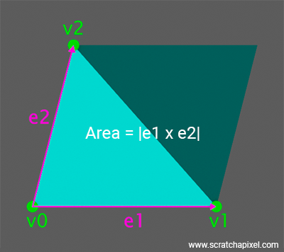
So the thing is that when, in the Sample method, we calculate the dot product between the sample direction d and the light normal, the light normal embeds, if you wish, the light area already. So the area, if you prefer, is effectively hidden in the light normal's magnitude, which is itself reflected in the result of the light sample direction-light normal dot product d_dot_Ng. Now, because the cross product magnitude of e1_ and e2_ is that of a parallelogram and not that of a triangle, we are only interested in half of that area, hence the factor 2 in the PDF calculation. So that explains why the area doesn't show up explicitly and why the 2 is in the code.

Now, what about tmax? The sample, thanks to the inverse square law, needs to be attenuated by the square of the distance between \(x\) and \(x'\). This is what two of these tmax account for. But why a third one? Because we do not normalize the direction d in the code. So the d_dot_Ng variable not only implicitly includes the magnitude of the light normal vector Ng_ but also the magnitude of the vector d. So we add an extra tmax in the denominator, which will effectively account for the vector d normalization. Okay, I agree we could have done things differently here since we still normalize d when calling the Sample3f constructor (wi = Sample3f(d / tmax, ...)), but hey, this is how you will see it in projects like Embree, and I am not responsible for their choices. The final term is the dot product of the angle between the light normal and the sample direction (see below). I rest my case.

If you want to look at the bigger picture, we could express things as follows:

With:

Substituting (we will switch from the equation variable names \(N_l\), the light normal, and \(w_i\), the light sample direction, to the code variable names, respectively Ng and d on the second line):

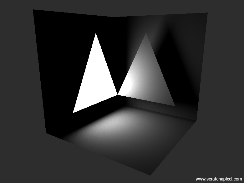
With \(|a|\) being the magnitude (length) of vector \(a\), and \(\hat{a}\) being the unit (normalized) vector of \(a\). So if you don't see the \(\hat{}\) (hat) sign over the vector's name, it means the vector isn't normalized. I hope this derivation clarifies the code. Wow! Congrats, pixel friends. You've made it. Compile, render, and here is what you will get (for all your effort). In the image below, we've used 2048 samples.

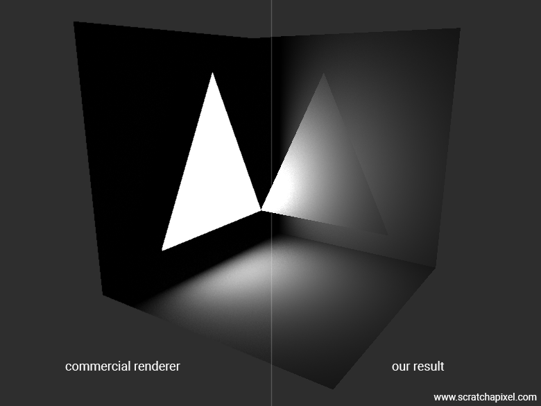
The commercial renderer has less noise than our render, but this is likely due to the fact that it uses a better solution for generating "random" numbers, which, as we have mentioned several times before, is something the lesson Sampling Strategies is devoted to. So overall, we have nothing to be ashamed of with this result. All we are left to do is plug in the code for the shadow rays to get our final result. This is easy; all we need to do is call the Occluded method to see whether the light sample is occluded or not.

Vec3f Li(const Ray& ray, const std::unique_ptr<Scene>& scene, bool debug = false) {
	...
	size_t num_samples = 2048;
	for (size_t i = 0; i < scene->lights_.size(); ++i) {
		Vec3f L_light = 0;
		for (size_t n = 0; n < num_samples; ++n) {
			LightSample ls;
			ls.L = scene->lights_[i]->Sample(dg, ls.wi, ls.tmax, Vec2f(rand() / (float)RAND_MAX, rand() / (float)RAND_MAX), debug);
			if (ls.L == 0 || ls.wi.pdf == 0 || dg.Ng.Dot(Vec3f(ls.wi)) <= 0.f) continue;
			bool in_shadow = [&]() -> bool {
				for (size_t i = 0; i < scene->num_triangles_; ++i) {
					if (Occluded(Ray(dg.P, ls.wi, dg.error * espsilon_, ls.tmax - dg.error * espsilon_), tris[i], vertices))
						return true;
				}
				return false;
			}();
			if (in_shadow) continue;
			L_light += 1 / M_PI * ls.L * dg.Ng.Dot(Vec3f(ls.wi)) / ls.wi.pdf;
		}
		L += L_light / num_samples;
	}

	return L;
}

As mentioned, for this example, we haven't used an acceleration structure and instead have opted to loop over all the triangles in the scene. This approach isn't typical for production code; we generally wouldn't use a C++ lambda function to calculate shadows or loop through every single triangle. However, in this instance, it serves our purpose for creating a concise, one-file implementation, resulting in a rather elegant solution—lambdas indeed rock.

Additionally, don't worry about the terms epsilon_ and df.error used in the code. If you're curious about their roles, particularly in avoiding self-intersections, you can check out the lesson on Avoiding Self-Intersection. The critical aspect here is that we've limited the shadow ray's range from near zero (essentially the value of epsilon) to tmax, which is the maximum distance for the ray. As you might suspect, there's no need to check for occlusion beyond the light source itself. Here is the result.

This Isn't the End of the Story: Cone Sampling and Better Sampling

The technique we've been using in this chapter relies on sampling the triangle's area. Before moving on to the next chapter, we just want to let you know that there's another possible technique that involves sampling the cone subtended by the triangle. We won't be studying this here because this chapter is long enough, but we've planned to address this topic in a future revision of this lesson. While it won't be specifically applied to triangles, you can still learn about uniform cone sampling in the chapter on spherical area lights.

As suggested above in the implementation section, it is important to note that alternatives to using two plain random numbers exist. These alternatives are presented in the lesson Sampling Strategies.

References

Graphics Gems - "Generating Random Points in Triangles" (p. 24), Greg Turk, Andrew S. Glassner, 1990.

A Low-Distortion Map Between Triangle and Square, Eric Heitz, 2019.