Introduction to Lighting

Point and Spot Lights

Reading time: 27 mins.

Sphere Light

Let's start with one of the simpler models: the point light. As the name suggests, a point light is a light source represented by a point in space. This type of light radiates equally in all directions and is part of what was mentioned in the previous chapter as the delta category and punctual light, which can be seen as a sub-category of the delta category.

Dealing with sphere light in CG is very straightforward since all we need to do to represent one in C++ is to create a point light class (which you can derive from a light class if you wish, this is a common approach) and add a variable to it (in addition to the light color and light intensity that are part of the light base class) to store the light position. This will be represented by a Vec3.

class Light {
public:
    virtual ~Light() = default;
    Vec3<float> color_{1.0};
    float intensity_{1.0};
};

class PointLight : public Light {
public:
    PointLight(Vec3<float> pos) : position_(pos) {}
    Vec3<float> position_{0.0, 0.0, 0.0};
};

As you can guess, when a primary ray intersects a surface and we want to determine whether the point is illuminated by our point light, all we need to do is cast a ray from $P$ the intersection point (or $x$ depending on the papers/books you are looking at) and use the point light position to define the shadow ray direction. From an implementation standpoint, we do this by passing the point light instance some information about the intersection point and letting the light fill up the data we need to cast our shadow rays. We will call this method Sample().

class Light {
public:
    virtual ~Light() = default;
    virtual Vec3<float> Sample(const DifferentialGeometry& dg, Vec3<float>& wi, float& pdf, float& t_max) const = 0;
    Vec3<float> color_{1.0};
    float intensity_{1.0};
};

At this point, we cannot explain why using the Sample() method is a good approach. We will discuss this in detail in the chapter on area lights. Don't worry too much about the variables within the Sample() method either. We will get to that in a moment. In this version of our program, we will store the information regarding the geometry at the intersection point in a structure called DifferentialGeometry. The structure looks like this:

struct Hit {
    float u;
    float v;
    int id0{-1};
    int id1{-1};
    float t{std::numeric_limits<float>::max()};
    operator bool() const { return id0 != -1; }
};

struct DifferentialGeometry : Hit {
    Vec3<float> P;
    Vec3<float> Ng;
    Vec3<float> Ns;
};

As you can see, it holds the intersection point P, and the geometric and shading normals Ng and Ns, respectively. The geometric normal is just the normal of the triangle itself, while the shading normal is the smooth shading normal, that is, the normal as specified at each vertex of the triangle weighted by the hit point's barycentric coordinates. We studied this technique in previous lessons. So once we find out that we have a hit for the primary ray, we will fill up that structure and pass it on to the light source Sample method:

DifferentialGeometry dg;
for (int i = 0; i < static_cast<int>(prims.size()); ++i) {
    const std::vector<Vec3<float>>& pos = prims[i]->position_;
    const std::vector<TriangleMesh::Triangle>& tris = prims[i]->triangles_;
    for (size_t j = 0; j < tris.size(); ++j) {
        Intersect(ray, dg, i, j, tris[j], pos.data());  
    }           
}
if (dg) {
    prims[dg.id0]->PostIntersect(ray, dg);
    Vec3<float> wi;
    float t_max, pdf;
    Vec3<float> light_L = light.Sample(dg, wi, pdf, t_max);
    // Further processing here...
}

This code snippet is part of the outer loop that iterates over each pixel in the image. What it does is that it tests each object making up the scene for an intersection with the primary ray (we loop over every object and every triangle of every object). If we find a hit (if dg returns true—you can see when this happens by looking at the implementation of the Hit structure above), then we call the PostIntersect method of the primitive that is responsible for setting dg.P, dg.Ng, and dg.Ns based on the hit data (using the primitive and triangle id that has been intersected as well as the s and t barycentric coordinates of the hit point on the triangle to interpolate the triangle vertex positions and normals). Once we get these set, we can then call the light Sample method with dg. Then, what we are interested in is what happens in that Sample method. Let's have a look.

class Point : public Light {
public:
	...
	Vec3<float> Sample(const DifferentialGeometry& dg, Vec3<float>& wi, float& pdf, float &t_max) const override {
		Vec3<float> d = position_ - dg.P;
		float distance = d.Length();
		wi = d / distance;
		pdf = distance * distance;
		t_max = distance;
		return color_ * intensity_;
	}
	...
};

**Figure 1:** A point light irradiates light in all directions. The direction to the light, $\omega_i$ is normalized. Any intersection with triangles that occurs at a distance greater than `t_max` can be ignored.

What you can see from the code is that we first calculate a vector d that extends from the intersection point dg.P to the light position position_. We store the distance between these two points into the variable distance for a reason we will explain soon. This distance is important. Then we set the vector wi as d divided by the distance, effectively normalizing the vector pointing towards the light position as seen from the point of intersection. We then set the pdf variable as the square of the distance, and the variable t_max to distance.

Why are we doing all this, and what are these wi, pdf, and t_max useful for?

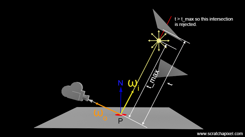
wi is a variable name we've already used in the previous chapter. It is the variable name most rendering applications, papers, or books use to designate the direction to the light. Note that this is not the direction from the light source to the point, but rather from the point to the light. This is always the case. While this might seem counterintuitive as it goes in the opposite direction to which light travels in the real world, we do this by mere convenience as it facilitates the calculation of things such as the dot product between the surface normal and the vector $\omega_i$. The same applies to $\omega_o$ as shown in Figure 1. As wi is a vector, it's being normalized—nothing unusual here.
t_max: we set our shadow ray's maximum distance to this value. The astute reader will have already noticed that, contrary to other lights such as the sun light which we will discuss in the next chapter, there's no point in casting a shadow that goes past the point light. For this reason, we will bound our shadow ray's parametric distance from 0 (not really 0, but more on this later) to t_max. This guarantees that while testing all triangles in the scene for an intersection, we ignore triangles for which the intersection lies beyond the light, as shown in Figure 1.
pdf: this one is a bit more peculiar to handle. The name pdf is poorly chosen for this one, but the pdf variable merely serves as a placeholder here for us to store the squared distance between the hit point and the light position. Why is the squared distance of interest to us? Well, we are touching upon a matter of primordial importance. For that, we will need to take a bit of space.

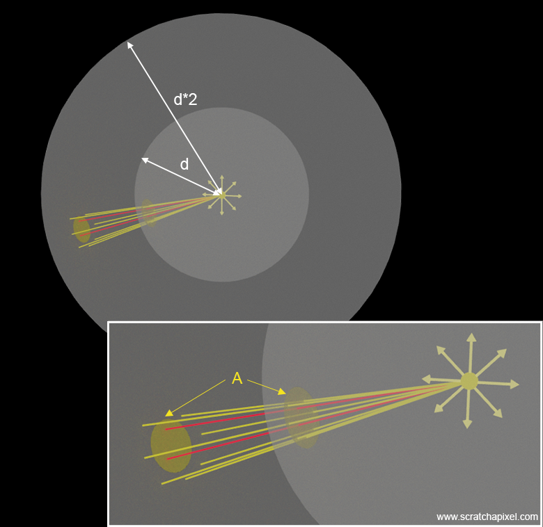
The reason we need the square of the distance is that there's a relationship between the energy received by a point illuminated by a light source and the distance between the point light source and that point. This becomes more understandable when we observe what happens to a series of 'light rays' emitted by a point light source as they travel through space. In Figure 2, we have represented only a few of these rays. Note that these rays are all contained within a small cone of direction intersecting an imaginary sphere with a radius $d$, centered on the point of emission. The intersection of the cone with the sphere defines a small spherical cap with area $A$. Now let's imagine an imaginary sphere whose radius is twice as large as the first one and see how many of these rays would now pass through a cone narrower than the first one so that its intersection with the larger sphere sustains a spherical cap with the same area $A$ as the area of the first cap. As you can see by looking at Figures 2 and 3, only a smaller number of these rays are contained within that cone when considering the larger sphere. We can intuitively deduce that the larger the imaginary sphere, the fewer the number of rays that pass through a spherical cap of constant area. What happens in reality is that for a surface area $A$, the ratio of this area to the surface area of the sphere is inversely proportional to the surface area of the imaginary sphere. And as you know, the surface area of the sphere is $4\pi r^2$ with $r$ representing the radius of the sphere. Thus, for a sphere with radius $r = 1$, we have a total surface area of $4\pi$. For a sphere with radius $r = 2$, the surface area of the sphere is $16\pi$. Thus, the surface area ratio between the two spheres is $1/4$. For a sphere with radius $r = 3$, the ratio between the first and the third sphere is $1/9$. Thus, we can see that the ratio is $1/r^2$. The ratio of energy for a constant surface area $A$ passing through a sphere centered around the point of emission is therefore inversely proportional to the square of the distance between the illuminated point and the light source, as we have shown in Figure 4.

**Figure 2:** The amount of light energy per surface area, here represented by just a few light rays, diminishes as the imaginary sphere centered around the light source increases in size. This image intuitively illustrates why the amount of incoming radiance from a point light source diminishes with the square of the distance between the point being illuminated and the source.

**Figure 3:** Same as Figure 2 but as a 2D view. You cleary see that an equal sphercical cap area, the number of rays passing through the cap decreases as the size of the imaginary sphere increases. THis is another illustration of the inverse square law.

This is known in computer graphics as the inverse square law and is something that we will be using almost constantly when dealing with lights. When the radius of an imaginary sphere centered around the light source doubles, the surface area quadruples because of the relationship between the surface area of the sphere and the radius squared ($4\pi r^2$). If $r$ doubles, the surface area through which the same amount of light is spread is four times larger, thereby making the light intensity one-fourth as much at twice the distance.

This is also referred to as the square falloff. Note that artists (if you are one) sometimes don't like or don't understand why using a square falloff on a point light source (and in fact, almost all light sources, except the sun) should be the norm. By not doing so, you're not following the laws of physics, and by not doing so, you cannot achieve physically accurate lighting. In other words, if you don't use a square falloff, your lighting will be incorrect, and it's likely you will be struggling with it in order to get a result that looks nice, particularly if you try to match the lighting of a live-action plate. Of course, some software (most of them) gives you the ability to turn it off or control the falloff exponent itself. However, we do recommend that you stick with the default and physically accurate behaviors and falloff values (which is the distance raised to the power of 2).

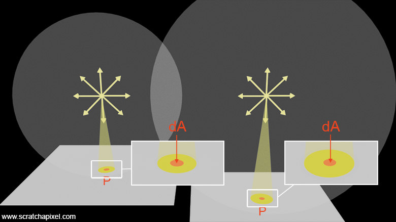
Before seeing the actual implementation of how light contributes to the illumination of our point, it's important to remember that while we've been representing light as rays in these illustrations, radiometry actually deals with solid angles. Consider a cone whose apex is located at the light origin; the profile of the cone becomes larger as the distance from the light source to the base of the cone increases. However, it's crucial to consider that the cone is, first of all, considered to be infinitesimally small. What we are really considering is the footprint of the cone on the surface, but within a small surface area $dA$ centered around point $P$ (or $x$). Therefore, one can develop another intuition about this square falloff by realizing that while the size of the footprint on the surface increases as the distance to the light increases, the ratio between the surface area $dA$ around $P$ and the footprint decreases (as visible in Figure 4). This effectively means that less light is being collected within $dA$ as the distance between the light and $P$ increases.

While I know my choice of variable name here might be a bit confusing, it's important not to mix up the differential area $dA$ that we just mentioned with the spherical area $A$ that we've been using before. The differential area $dA$ relates to the surface being illuminated, specifically, the surface of the object. It's a differential area centered around the point of illumination. We do so in rendering because, like everything else, the real-world is not made out of infinitesimally small points, but is continuous. Thus, our equation needs to function with surfaces rather than points, which have no physicality. Though we understand that over a surface the intensity of light impinging on that surface might vary, which is why we always take a super small surface area $dA$, considering it so small that over that area, we assume the lighting impinging on its surface is constant. While one might argue that this is another construct of the mind, no more valid than using infinitesimally small points, which I can understand, the former has yet more physical/mathematical grounding than the latter. And yet, yes, $dA$ is a mind construct since we don't really specify what size this thing is; we just assume that it is small enough that the maths that "decouples" from using it are "correct and sound". As for $A$, this relates to the surface area of the spherical cap defined by the intersection of a cone of direction with an imaginary sphere centered around the point light. Note that both $A$ and $dA$ are related to each other because in radiometry, what we're really considering is how this spherical cap projects onto the object surface around $P$. This is where Lambert's cosine law comes into play, as it defines that the amount of light projected from $A$ into $dA$ (in short, how much of $dA$ is subject to receive light from $A$) is proportional to the cosine between the surface normal and the light direction (cone orientation).

**Figure 4:** Another way of understanding the square falloff is to realize that the size of the cone footprint, when thought of in terms of solid angle, gets larger as the distance between $P$ and the light source increases. This means that the ratio between $dA$, the infinitesimally small area around $P$, and the cone footprint on the surface, decreases as this distance increases. Consequently, less light is being 'collected' by $dA$ as the distance increases, explaining the falloff.

Now you understand why we need the squared distance. As suggested, we store this value in the pdf member variable. Not a great choice, but the reason we have a variable called pdf will be explained when we get to area lights. For now, just remember that what the pdf variable holds in the case of the point light source is the distance to the light source squared. Let's use the data set in Sample() to calculate the contribution of this light to our point. Here is the code:

if (dg) {
    prims[dg.id0]->PostIntersect(ray, dg);
    Vec3<float> wi;
    float t_max, pdf;
    Vec3<float> light_L = light.Sample(dg, wi, pdf, t_max);
    bool in_shadow = Occluded({dg.P, wi, 0.01f, t_max - 0.01f}, prims);
    if (in_shadow)
        continue;
    Vec3<float> L = light_L * std::max(0.f, dg.Ns.Dot(wi)) / (M_PI * pdf);
    pbuf[0] = static_cast<uint8_t>(std::min(1.f, L.x) * 255);
    pbuf[1] = static_cast<uint8_t>(std::min(1.f, L.y) * 255);
    pbuf[2] = static_cast<uint8_t>(std::min(1.f, L.z) * 255);
}

After calling Sample(), we use the light vector to cast a shadow ray. This is done by a call to Occluded, which is similar to Intersect() but, as mentioned earlier, is optimized for shadow rays. Remember, we can return from the function as soon as we have found one valid intersection. A valid intersection is one that occurs within a distance from $P$ that is less than t_max, the distance from $P$ to the light source. Check the code on GitHub to see the differences in implementation between Intersect() and Occluded(). Then, if $P$ is in shadow, the light doesn't contribute to the illumination of $P$ and we then skip the rest of the code block. If the point is not in shadow, we set L, the radiance at point $P$, as the light intensity multiplied by the light color (light_L, which is returned by Sample()) multiplied by the dot product between the surface normal and the light direction -- our famous Lambert cosine term -- divided by $\pi$, the normalization factor of a diffuse surface, and the pdf parameter, which holds the squared distance from $P$ to the light.

We can formalize this with the following equation:

$$ L = \color{red}{f_r(\omega_o, \omega_i)} \color{blue}{\times \frac{I}{d^2} \times (N \cdot \omega_i)} $$

Where:

$f_r(\omega_o, \omega_i)$: This should technically be our BRDF (which we discussed in the previous chapter). For a purely diffuse surface, this should be $\frac{\text{albedo}}{\pi}$, as explained in the lesson 'A Creative Dive into BRDF, Linearity, and Exposure'. Generally, BRDF models use the incoming light and outgoing view directions, but diffuse materials reflect light in every direction regardless of its incoming direction, and consequently, for these types of surfaces, $\omega_i$ and $\omega_o$ can be ignored.
$I$: is the light intensity, which combines its color and intensity, as coded.
$d$: is the distance from $P$ to the light. And, thanks to the inverse square law, we need to square this distance.
$N$ and $\omega_i$: are respectively the surface normal and the light direction. The last term in the equation (the dot product) represents the Lambertian cosine law.
$L$: stands for our outgoing radiance. This is the light that has interacted with the surface and is being reflected or scattered back towards the observer. It depends on the properties of the surface material (modeled by the BRDF), the incoming light (its intensity and direction), and the geometry of the surface (normal and viewing direction).

You might see BSDF (Bidirectional Scattering Distribution Function) besing instead of BRDF (Bidirectional Reflectance Distribution Function) sometimes. BSDF is more general than BRDF, but generally, they mean the same thing. BSDF accounts for both surface reflection and transmission, whereas BRDF only accounts for reflection. You can see BRDF as a subset of the BSDF case.

Once you have calculated L in the code, you just need to convert the floating-point value to a range within [0, 255] and store the result into the image buffer at the current pixel location. That's it. Note that we assume in the code above that the object's albedo is white, and so it's not explicitly defined. However, note the division by $\pi$ in the code. Since the object's albedo is white, all we need is to multiply the blue part of the equation by $\frac{1}{\pi}$. The following image shows the output of the program (left) compared to the same scene rendered in Maya with Arnold (right). As you can see (and hopefully so), the two images match perfectly. Maths never lie.

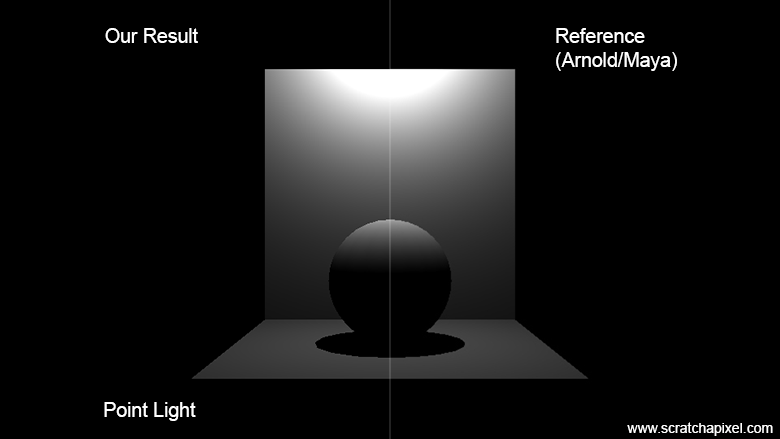
The complete code of the program that was used to produce that image can be found on the GitHub repo (use the link from the table of contents at the top of the page).

The following video shows how the shape of the shadows changes as the sphere gets closer to the surface. To understand why the shadow gets bigger as the point source moves closer to the sphere, we have represented the projection of the sphere onto the plane as a triangle, as seen from the source. The fact that the shadow size changes with the proximity of the light source to the geometry is an important visual cue that differs with distant light, as we will explain in the next chapter. Note also how the surface gets brighter as the point light source gets closer. This is due to the inverse square law: the smaller the distance to the source, the more light impinges on the surface at any point whose illumination is being calculated.

The astute reader may again ask themselves what happens when that distance is less than 1? Indeed, dividing the light intensity by a value approaching zero should lead to resulting values approaching infinity! That's clearly not physically accurate. Well, this is where we pay the price for our model's simplicity. As mentioned in the previous chapter, point lights do not have a physical size, unlike any real-world light source. The lack of size means that while the model works well when the distance to the light source is greater than 1, it fails at accurately simulating light interaction as the distance approaches 0. For more accurate modeling, you would need to use a different model that either simulates a physical size for the sphere or just use geo lights (or area lights, which are simplified versions of geo lights). We will cover that in the chapter on area lights. Note that some applications, notably video game engines, address this problem (though they don't really solve it per se) by capping the distance squared like so:

$$\dfrac{I}{\max(d^2, 0.01^2)}$$

Feel free to do the same if you want to. Another approach that some game engines take is to add a radius of influence to point light sources. The issue with these light sources is that even though their contribution can be very small when far away, they still need to be computed within the light loop. If you have 10 lights and only 1 of them significantly contributes to the scene while the others are too far to make a visual difference, 9 of them induce a computation penalty that we would be happy to avoid if possible. So one way to solve this problem is to add a sphere of influence beyond which we decide that the light doesn't contribute to the illumination of point $P$. A common formula being used is the following:

$$\dfrac{I}{\max(d^2, 0.01^2)} \left ( 1 - \dfrac{d^4}{r^4} \right)^2$$

Where $r$ is the radius of influence of the point light. What happens is that light contribution quickly drops off to 0 as $d$ gets close to $r$. We won't be using this method in our code, but we are just mentioning it here for the sake of completeness.

Spot Light

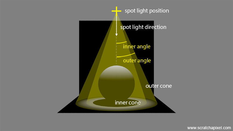
Once we understand how to implement point lights, implementing spotlights becomes straightforward. Indeed, spotlights are essentially a subset of point light sources. You can envision a spotlight as a cone whose apex is at the position of the point light, as shown in Figure 5. Like point lights, spotlights are defined by their location, color, and intensity parameters, which are common to all lights. Additionally, we define two parameters: one to specify the aperture of the inner cone and another to specify the aperture of the outer cone, defined respectively as the inner and outer cone angles (Figure 5). The bounded area defined by the two cones allows control over the light falloff, with the intensity diminishing between the inner and outer cones. Since the projector can also be arbitrarily oriented around its position, we need to add a direction vector. Ideally, it's best to define the projector's default direction (generally (0,0,-1), similar to the default position and orientation of cameras) and use a 4x4 transformation matrix to control the spotlight's orientation (and position).

Since spotlights are subsets of point lights, here again, we will need to apply the inverse square law (obviously).

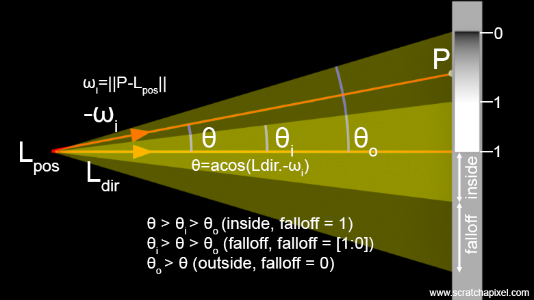
The mathematics behind simulating a spotlight are a bit more involved than those for a point light, but nothing too complicated. We need to determine whether the ray connecting $P$ to the light source falls within the falloff region. To do this, we calculate the dot product between the spotlight direction and $\omega_i$, the normalized vector from $P$ to the light. Note that the light direction and $\omega_i$ point in opposite directions, since $\omega_i$ goes from $P$ to the light source (as shown in Figure 6). Thus, we can either negate the light direction or negate the result of the dot product (we will choose the latter). Remember that the dot product between two vectors is equal to the cosine of the angle between them:

If the vectors are pointing in the same direction, the dot product is 1. The angle between the vectors is 0, and $\cos(0) = 1$.
If the vectors are perpendicular to each other, the angle between the vectors is 90 degrees, and $\cos(90) = 0$. This also implies that the outer and inner angles of the spotlight cannot be greater than 90 degrees.

Now, to determine whether $P$ is inside the inner cone, outside the outer cone (where no light is received from the spotlight), or in between (in the falloff region), all we need to do is compare this dot product against the cosines of the inner and outer cone angles:

If the dot product between the light direction and $\omega_i$ (or rather $-L \cdot \omega_i$, as mentioned above—don't forget to negate the result) is higher than the cosine of the inner angle, then $P$ is within the inner cone and receives full illumination without any falloff.
If the dot product is less than the cosine of the outer angle, then $P$ is outside the outer cone and no contribution is received from the light.
For any dot product within the two cosines, $P$ is in the falloff region. Here, all we need to do is remap the dot product from 1 to 0 (1 at the edge of the inner cone and 0 at the edge of the outer cone). This is a simple linear remapping problem, which we achieve using:

$$\text{attenuation} = \frac{(-L \cdot \omega_i - \cos(\theta_o))}{(\cos(\theta_i) - \cos(\theta_o))}$$

Where:

$\theta_i$ is the inner cone angle.
$\theta_o$ is the outer cone angle.
$L$ is the light direction.
$\omega_i$ is the normalized vector from $P$ to the light position.

Remember that $\cos(\theta_i)$ is greater than $\cos(\theta_o)$ since $\theta_i \leq \theta_o$. When you want to normalize a value (remap a value from the range $[lo, hi]$ to the range $[0, 1]$), the equation is:

$$V_{\text{Normalized}} = \frac{V - lo}{hi - lo}$$

This formula adjusts the value $V$ so that when it is at the lower bound of the original range ($lo$), it maps to 0, and when it is at the upper bound ($hi$), it maps to 1. Don't forget to clamp this value in the range [0:1]. In code, this would be implemented as:

float cos_inner_angle = std::cos(inner_angle); // in radians
float cos_outer_angle = std::cos(outer_angle);
float falloff = std::clamp((-light_dir.Dot(wi) - cos_inner_angle) / (cos_inner_angle - cos_outer_angle), 0.f, 1.f);

**Figure 6:** We calculate the angle between the light direction and $\omega_i$ to compare this value against the angles $\theta_i$ and $\theta_o$. Note that in the image, we've been using angles for comparison, but in practice, it suffices to use the dot product between the two vectors, which is equal to the cosine of the angle.

Here is the complete code for the Sample() method of our SpotLight class:

class SpotLight : public Light {
public:
	SpotLight(float angle_inner = 20.f, float angle_outer = 25.f) {
		cos_angle_inner_ = std::cos(DegToRadians(angle_inner));
		cos_angle_outer_ = std::cos(DegToRadians(angle_outer));
	}
	Vec3<float> Sample(const DifferentialGeometry& dg, Vec3<float>& wi, float& pdf, float &t_max) const {
		Vec3<float> d = pos_ - dg.P;
		float distance = d.Length();
		wi = d / distance;
		pdf = distance * distance;
		t_max = distance;
		float falloff = std::clamp((-wi.Dot(dir_) - cos_angle_outer_) / (cos_angle_inner_ - cos_angle_outer_), 0.f, 1.f); 
		return color_ * intensity_ * falloff;
	}
	Vec3<float> pos_{0,0,0};
	Vec3<float> dir_{0,0,-1};
	float cos_angle_inner_;
	float cos_angle_outer_;
};

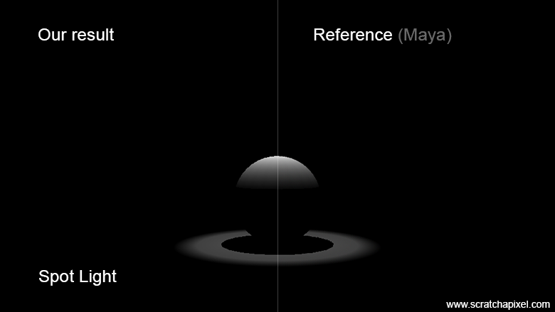
Surprisingly simple, right? Here is the result, which, as expected, is similar to what other production renderers produce. Note that you might see differences with other rendering engines, which can be attributed to how they've decided to implement the falloff. This is the case with the Arnold renderer, for instance, which shows a result different from what the Maya native renderer produces.

Note that in the implementation of the spotlight, we've decided to use a matrix to rotate the light from its default direction (0,0,-1) to the desired direction: in our case, (0,-1,0), which required a rotation of -90 degrees along the x-axis. We've set the light position directly, though. In a production renderer, you should use the light transformation matrix to set both the light direction and position. We haven't done this in our demo just to show different ways of achieving the same goal.

SpotLight light;
Matrix44<float> m;
m.SetAxisAngle(Vec3<float>(1,0,0), DegToRadians(-90));
m.MultDirMatrix(light.dir_, light.dir_); // set the spotlight direction
light.dir_.Normalize();
std::cerr << "Spotlight direction: " << light.dir_ << std::endl;
light.pos_ = Vec3<float>(0,6,-22); // set the spotlight position, could have used the matrix as well

Note that some engines also like to square the falloff, as shown here:

Vec3<float> Sample(const DifferentialGeometry& dg, Vec3<float>& wi, float& pdf, float &t_max) const {
	...
	return color_ * intensity_ * falloff * falloff;
}

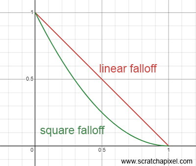
**Figure 7:** Squaring the falloff values can help produce a more subtle and gradual falloff effect.

This approach has no real physical justification but can provide a falloff that feels more natural and is thus more pleasing to the eye, as it makes the transition from light to dark more gradual and subtle. Figure 7 illustrates the difference. Be mindful not to confuse this type of falloff with the inverse square law "falloff." While on this topic, note that the code for adding up the contribution of the spotlight is not different from the code used for the point light. We multiply the light intensity (a mix of color, intensity, and falloff here) by the dot product (cosine) between $\omega_i$ and the surface normal, divided by $\frac{1}{\pi}$ for the BRDF (assuming the object's albedo = 1 in this case, and the $\pi$ factor accounts for the normalization required when dealing with diffuse surfaces as explained above) and the square of the distance (stored in the variable pdf) from $P$ to the light.

Vec3<float> L = light_L * std::max(0.f, dg.Ns.Dot(wi)) / (M_PI * pdf);

Conclusion & Takeaways

This concludes our chapter on implementing punctual lights. So far, it hasn’t been too difficult, but you’ve learned a critical aspect of lighting in this chapter, which is the inverse square law. In the next chapter, we will learn how to implement another type of delta light: the distant light. Before we go, let's pay a quick tribute to Pixar, who used spotlights creatively in their revolutionary short animated film Luxo Jr., produced in 1986.