Introduction to Lighting

Area Lights: Mathematical Foundations

Please Read: A Word of Warning

Area lights are more complex to implement than point, sun, and spot lights. Even though they might seem ubiquitous these days to those who haven't experienced the early days of computer graphics, this was not always the case. Ray-tracing allows for a more "precise" evaluation of area lights' contributions compared to alternative methods primarily based on shadow maps. However, the flip side is that ray-tracing is inherently slow. As Kajiya once said, it's not that ray-tracing is slow; it's the computers. Given that computer power has significantly evolved since Kajiya's era, ray-tracing remains computation-intensive, but now machines can handle the task within reasonable times, facilitating its widespread adoption in production in recent years.

However, despite the best computer performances allowing a generalization of ray-tracing-based rendering, the mathematics involved in evaluating the contribution of area lights to illuminating a 3D scene is also more complex than the math for point or spot lights. As a result, we will need to cover much more material to give you an overview of how it works. The concepts covered from this point may require long and sometimes complex explanations, and since this is only meant to be an introductory lesson, we face the challenging exercise of providing enough information without being overly long, too technical, or merely repetitive of lessons where these concepts are detailed. We apologize in advance, but as I've said, this is a difficult task, and the lessons from Scratchapixel often overlap. Our learning method is generally to re-explain a technique within the context of this lesson, even if the technique itself is part of a dedicated lesson. That's just how it goes. Ideally, each lesson should function independently of the others, as much as possible. So, please keep this in mind and stay engaged as much as possible while reading the following chapters.

Honestly, we believe this lesson is one of the best resources available on the subject, especially for an audience relatively unfamiliar with the mathematical concepts presented in this lesson. We've tried to present them as usual with simple words, clear examples, and by breaking down the demonstrations into as many steps as possible. So while this may seem like a lot of effort to go through, I really believe it's worth the pain, particularly considering that you won’t find many places where this will be as well explained and illustrated. 'All great achievements require time.'

Why Are Area Lights Ideal?

Punctual lights are still widely used in production, especially in video games, due to their simplicity and relatively low computational costs compared to ray-traced area lights (and even shadow-map based techniques, which themselves suffer from severe limitations). However, they inherently suffer from conceptual flaws which make them unable to accurately reproduce real-world lighting scenarios. Let’s review these limitations to better understand why area lights should ideally be used whenever possible.

As suggested, the intrinsic flaw of punctual lights is their lack of size, which leads to a series of problems. The two main issues are:

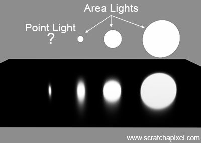
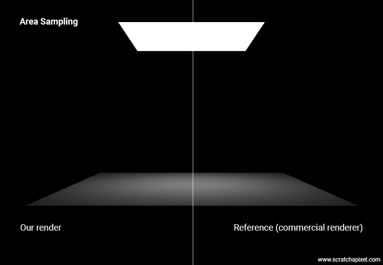
• Reflection of punctual light sources is not physically realistic: We "see" objects because light is reflected from either objects that are illuminated by other light sources (indirect lighting) or from the light sources directly (direct lighting). Objects in a scene have a size, so simulating their reflection onto other surfaces is generally straightforward. However, indirect specular or diffuse reflection only became feasible when computers were sufficiently powerful to handle them within reasonable timeframes (ranging from a few minutes to a few hours). For more details on these techniques, particularly for diffuse reflections, see the lesson Global Illumination and Path Tracing. But if lights have no size, how can they reflect onto a surface?

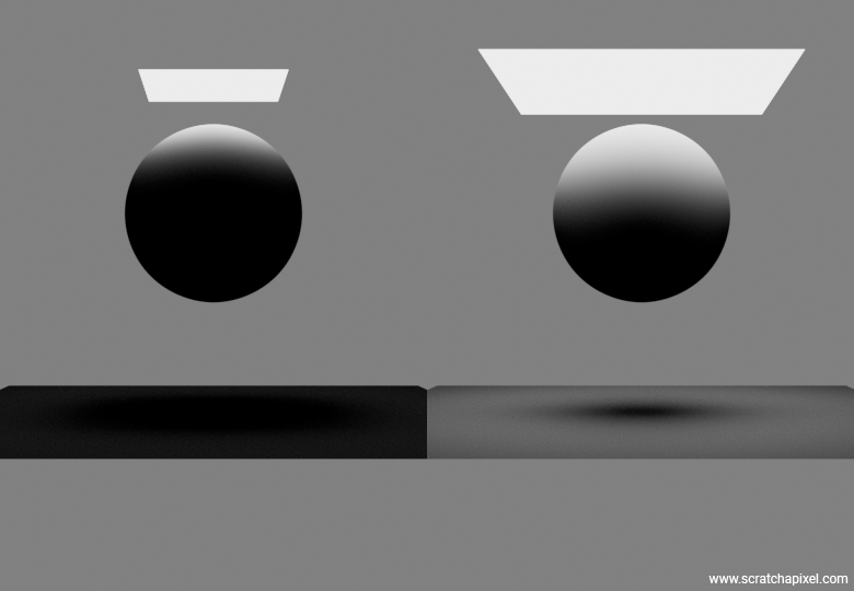
  In the adjacent image, you can observe the reflection of three area lights on the surface of a plane, where the size of their reflection is proportional to the size of the light represented in the scene as a 3D object (in this example, a simple disk). To the left of the image, the light used is a point light. While a reflection of this light is visible on the surface of the plane, the size of this reflection does not correspond to physical reality. The reasons why the specular reflection of this light is visible are discussed in the lesson Introduction to Shaders and BRDFs. Thus, although we see a reflection, it lacks physical realism and its size cannot be controlled, posing challenges when the goal is to create images that simulate reality.

  

• Punctual Lights do not generate soft shadows by design: The video below demonstrates how the size of an area light influences the size of the penumbra projected onto the floor by the light due to a blocking sphere. The smaller the light, the sharper the shadow. Conversely, the larger the light, the softer the shadows. Since punctual lights have no physical size, they are inherently designed to produce perfectly sharp shadows, which is often undesirable for realistic rendering.

As mentioned before, pioneering researchers laid the mathematical foundations for simulating ray-tracing with area lights early on (late 1970s/early 1980s). However, computers at that time were not powerful enough to handle these calculations within a reasonable timeframe. It wasn't until the late 2000s/early 2010s, when computers became sufficiently powerful, that ray-traced area lights started being feasibly used in production without being prohibitively expensive. This is particularly true since it has become easier to run ray-tracing on GPUs (around 2016 with the release of RTX-based GPUs by Nvidia and AMD), which prior to this innovation was limited to CPUs (attempts to use GPUs for ray-tracing date back to roughly the mid-2000s).

The rest of this chapter will be devoted to introducing the mathematical concepts involved in understanding how to simulate area lights with ray-tracing, which, as suggested, is both more straightforward than alternative techniques (notably shadow-map techniques or radiosity methods) and does not suffer from the limitations these techniques have. But since nothing is ideal in this world, of course, we will see that ray-traced area lights have their own drawbacks!

A Quick, Friendly Introduction to the Concept of Monte Carlo Integration

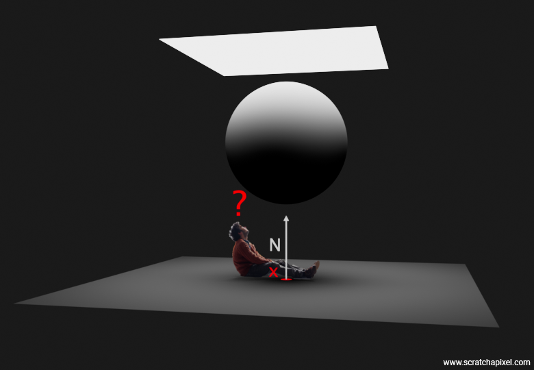
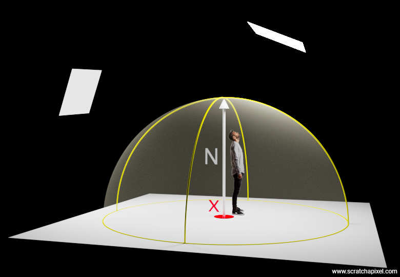
Let's put ourselves in the shoes of a point being illuminated by an area light. Imagine you are this point, as shown in Figure 1. Considering your normal, you are looking straight up, and what you see is essentially a sphere partially blocking the surface of the area light. From this perspective, it’s not hard to guess that only a fraction of the light emitted by the area light will illuminate you, since part of the light is blocked by the sphere

Your task is to measure "how much of the light that is emitted across the entire surface of the light is being blocked by the sphere?" The sphere has some nice geometrical properties, so you might think you could exploit those to calculate the ratio of light emitted to light blocked, but that would be too simple. No, your task is to devise a method that will work regardless of the shape blocking the area light, which could range from another plane, a sphere, to a rabbit or even a unicorn if the director has decided so. Remind me to tell you the story one day about those famous film directors who once requested a CG set be covered with pink windmills just a few days before the film’s release date—a true story! So, why not a unicorn? So how do we do that?

Imagine a white image of 512x512 pixels with a black disk of radius 128 pixels centered in the image. This setup represents the area light as viewed from our point \(x\), with the dark disk in the center symbolizing the sphere that blocks the light as seen from \(x\). To solve our problem, we'll employ a radiosity-inspired approach that involves subdividing the image by splitting it into two along every dimension. This results in four quadrants on the first iteration. We continue to subdivide these quadrants until we reach a maximum subdivision level, or when a quadrant is either entirely within or outside of the sphere. A quadrant overlaps the sphere if it contains both white and black pixels. In the end, we will sum the number of pixels in quadrants filled exclusively with white pixels (excluding those that overlap the sphere or are contained within it). Then, we will divide this number by the total number of pixels in the image to determine the unblocked portion of the light.

Before we look at the results in Figure 2, note that using mathematics, we can very precisely calculate the ratio between the part of the light that is not blocked by the sphere. Since we know the disk radius, we know the total number of pixels covered by the sphere is exactly \(\pi \times r^2\) or \(\pi \times 128^2 = 51,471.85\). We now take the ratio between that number and the total number of pixels in the image, which gives us \(\frac{\pi \times 128^2}{512^2} = \pi \times \frac{1}{16} = 0.1963\). So, 19.63% of the area light is occluded by the sphere, which means 80.37% of the area light is visible to \(x\). That's the way by which we can calculate this number analytically. Let's call this number (80.37%), our expected value.

Now, let's see the results. As you can see in the animation of Figure 2, the ratio approaches 80.37% as the number of subdivisions increases. So, this technique works, and we can see that by subdividing our quadtree more, we can improve the estimation. Note that while we have been doing this with a sphere as the occluding object, this technique could work with any shape. Good.

Remember, what we're attempting to determine here is how much of the area of the light is visible to \(x\). This can be formulated—mathematically speaking—as an integration problem. Such problems involve summing or integrating values across a space or surface (like the surface of the area light)—referred to as the domain of integration—to determine an overall measure, such as visibility, area, or intensity of an area light. We've previously tackled this using the radiosity-inspired space subdivision method. However, now we'll employ another method known as Monte Carlo integration.

I won’t delve into the details about the mathematics behind these methods since there are a series of lessons on the website that go into great detail on this very topic (see for example Mathematical Foundations of Monte Carlo Methods and Monte Carlo Methods in Practice). Since they are essential for understanding the implementation of ray-traced area lights, we will have to cover much ground already explored in these lessons. Apologies for the repetition; however, what's great about this is that the way we are going to introduce these concepts in this lesson is somehow much more friendly than the approach taken in the two lessons devoted to Monte Carlo methods, and they are certainly very complementary as well. To start, we will start with a very simple and informal but practical examples, and fomralized the concepts from there.

The idea with this Monte Carlo integration method, which is based on probability (more on that later), involves sampling the surface of the area light. Measuring the average height of the adult population of your country by measuring the height of every adult and dividing the sum of these heights by the total number of adults is probably not practical. Instead, you could measure the height of a few thousand people randomly selected from the adult population of your country, measure the heights of these selected individuals, and then average the sum of these heights by the size of your sample. This won't give you the exact average weight of the adult population, but statistically, it will provide a reasonable approximation. This is the concept behind polls used in pre-election times. Similarly, we can apply this method to area lights. Imagine throwing beans randomly onto the surface of the light—a process akin to selecting random people from your country's adult population—and counting how many beans have fallen inside or outside the disk (the disk represents the objects potentially occluding the light from point \(x\)). Mathematically, this is straightforward: we create random points over the surface of our 512x512 image, check if each point is inside or outside the sphere, and if outside, we increment a counter. Once we have created all the points we want, we divide the total number of beans outside of the disk by the total number of beans. Here is some Python code that will do just that:

import numpy as np
import matplotlib.pyplot as plt

def draw_disk(image, center, radius):
    for x in range(image.shape[0]):
        for y in range(image.shape[1]):
            if (x - center[0])**2 + (y - center[1])**2 <= radius**2:
                image[x, y] = 0  # Black for inside the disk

def is_inside_disk(center, radius, point):
    return (point[0] - center[0]) ** 2 + (point[1] - center[1]) ** 2 <= radius ** 2

# Initialize parameters
width, height = 512, 512
radius = 128
center = (width // 2, height // 2)
num_points = 128

# Create a white image
image = np.ones((width, height)) * 255

# Draw a black disk
draw_disk(image, center, radius)

# Monte Carlo simulation to estimate the area outside the disk
outside_count = 0
points = np.random.randint(0, high=width, size=(num_points, 2))

# Set up the plot
fig, ax = plt.subplots()
ax.imshow(image, cmap='gray', origin='upper')

# Check each point and adjust markersize
for point in points:
    inside = is_inside_disk(center, radius, point)
    if not inside:
        outside_count += 1
    color = 'ro' if inside else 'go'
    ax.plot(point[1], point[0], color, markersize=3)  # Smaller point size

# Calculate percentage of points outside the disk
percentage_outside = (outside_count / num_points) * 100

# Display the result
ax.set_title(f"Monte Carlo Estimation of Area Outside Disk: {percentage_outside:.2f}%")
ax.set_xticks([])
ax.set_yticks([])

plt.show()

Figure 3 shows results for an increasing number of points, specifically: 128, 256, 512, 1024, and 2048. As you can observe, similar to the radiosity-based method, the more points or samples we use, the better our estimation becomes—or to be more precise, the probability of approximating the expected result improves, but we'll discuss that more later. This result is really surprising. By simply randomly throwing beans and counting the number of these beans that do not overlap the occluded area, we can estimate the visibility integral. This method is incredibly simple and yet efficient.

Note that in the last image, where we've used 2048 samples, the result (81%) exceeds the expected value (80.37%). With Monte Carlo methods, results may sometimes fall below or rise above the expected result. The difference between the estimation and the expected value is referred to as variance. Since the result of the estimation depends on our sample selection, which is random, changing the seed of the random number generator could lead to entirely different results for the same number of samples, with some results being above, below, or exactly equal to the expected value. The specific outcome—whether it's one of these three possible positions—is unpredictable since it depends on a random process: the selection of samples. Whether the estimation is above or below the expected value is not critical. What matters is that as the number of samples increases, the probability of achieving a result close to our expected value also increases (as would be observed if we continued our simulation with an ever-increasing number of samples). A detailed explanation of this method can be found in the lesson Monte Carlo Methods. In short, the variance is likely to be less with 2048 samples than with 16 samples. Our confidence that the estimation approaches the expected value increases as the number of samples increases.

This example has hopefully given you an intuition into what Monte Carlo methods are and how they work—by evaluating a given function (the area light visibility) at random samples over the domain of integration (the surface of the light), and averaging the results of these samples by the total number of chosen samples.

Let's raise the difficulty a notch.

The Rendering Equation and Hemisphere vs Area Sampling

To further our exploration of area lights, we need to take a step back and examine how we simulate the effect of lights in computer graphics. This will lead us to present one of the most important equations in rendering, known as the rendering equation. For now, we will present a simplified version limited to diffuse-only surfaces. While a complete lesson on this advanced topic is devoted to the rendering equation, we cannot ignore this crucial concept here, which we need in order to delve into the challenges of implementing area lights.

The principle of this equation is not too complicated. Imagine you are a point. Below you is an opaque surface. Therefore, light illuminating you cannot come from below. It must come from above, and since the plane you are sitting on divides the space into two, the light coming from above is necessarily contained within a hemisphere of directions centered around the normal at the point where you are situated. This concept is pretty straightforward and is illustrated in Figure XX, where you can see the hemisphere oriented along the normal at \(x\). Here, light illuminating \(x\) comes from the two area lights we've added to this simple scene.

As you may have guessed, we want to "integrate" (a synonym for 'collect') the amount of light coming from the hemisphere of directions. This presents an integral problem because, although the hemisphere is purely virtual, it is a surface—at least, you'll agree, it is not made out of discrete elements. Now, in computer graphics (and in physics), when we come to integrate over a set of directions (here, the hemisphere), we deal with the concept of solid angle (which is the counterpart of the differential area we have already discussed in the previous chapter—as with the concept of solid angle, which was also introduced then). Solid angle can be thought of as a representation of an area, if you wish, over the unit sphere (or hemisphere, in our case). Its unit is the steradian. The surface of a sphere being \(4\pi r^2\), and considering we are dealing here with the unit sphere (well, the hemisphere, not the sphere), our hemisphere has \(2\pi\) steradians.

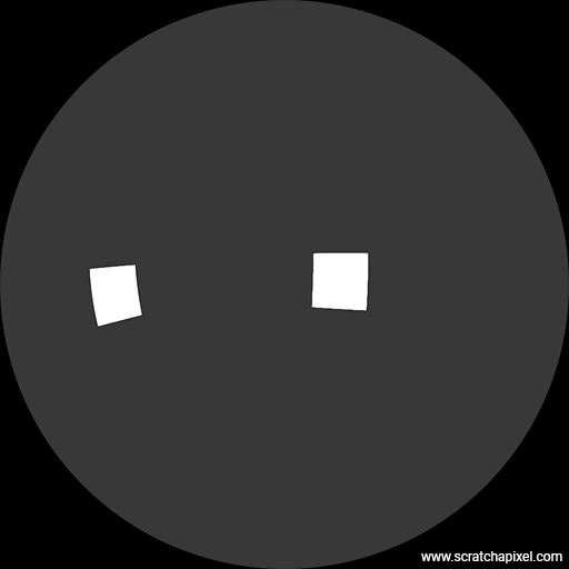
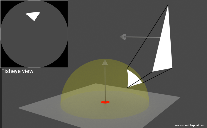
To put it another way, or to visualize it if you prefer, consider the figure below that shows a 180-degree fisheye view of the scene as seen from \(x\). This is essentially what \(x\) "would see," and all light arriving at \(x\) would come from what "it sees." What we need to do is "scan" through that view and collect light. However, since it's a continuous space, we must resort to integration to represent this process mathematically.

The rendering equation—perhaps one of the most famous equations in computer graphics—performs this task for us. It integrates the amount of light arriving at \(x\) from within a hemisphere of directions. This light is multiplied by the surface BRDF and the Lambert Cosine Law for every direction considered over the hemisphere. The integrand—the function that's being integrated—is the amount of light arriving at \(x\) from every possible direction within the hemisphere (the \(Li\) term below). It can be defined as follows:

Where:

• \(L(x)\) is the radiance (color) of \(x\),

• \(Li(x, \omega)\) is the light coming inward toward \(x\) from direction \(\omega\),

• \(\theta\) is the angle between the surface normal at \(x\) and the light direction,

• \(\cos(\theta)\) is, as stated before, the application of the Lambert cosine law (a weakening factor of outward irradiance—the incoming amount of light—due to the incident angle).

You could look at the \(\textcolor{orange}{Li(x, \omega) \cos(\theta)}\) term as the illumination part of the equation. I left four terms in there so that you pay special attention to them:

• \(\textcolor{blue}{\frac{R(x)}{\pi}}\) is technically a representation of the BRDF. In this lesson, we only deal with perfectly diffuse surfaces, and \(\frac{R(x)}{\pi}\) describes the BRDF of a diffuse surface. Here, \(R(x)\) represents the surface albedo (also sometimes denoted by \(\rho\), the Greek letter rho)—think of it as the surface color, if you prefer. The \(\pi\) in the denominator acts as a normalizing factor (see the lesson on BRDF for a detailed explanation). Although this term would conventionally appear on the right side of the integral, it can be moved out of the integral to the left because it is a constant in this context.

• \(H^2\) represents the domain of integration which is the hemisphere in this case. The Greek letter \(\Omega\) (Greek upper case letter "omega") is also sometimes used.

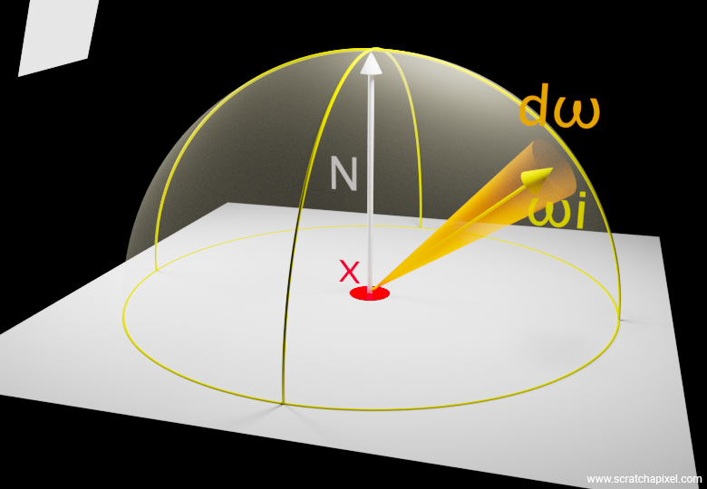
• \(d\omega\) is what we call the differential solid angle. In mathematics, we call this the differential of the variable \(\omega\) (in this case) and it indicates that the variable of integration is \(\omega\).

• \(\omega\) itself, which we need to consider, is the negative direction of the incoming light being considered.

The following figure attempts to represent how one of these "directions" in the integral can be visualized. You can think of it as a small cone starting from \(x\) and oriented along the incoming light direction \(\omega\). Note again that the small cap this cone would form on the surface of the unit hemisphere is the counterpart to the concept of differential area, which we discussed in the lessons devoted to BRDFs.

The rendering equation is solved by integrating the amount of light incoming at \(x\) within a hemisphere of directions. The integrand—the function that's being integrated—is the amount of light arriving at \(x\) from every possible direction within the hemisphere. We solve this using Monte Carlo integration, which is exactly how we've addressed our "ratio of visible light surface" problem above. We will sample our domain of integration, which is the surface of the hemisphere, by choosing a number of directions randomly, shooting rays along these directions, and checking if they intersect an object emitting light, such as an area light (for this lesson, we will limit ourselves to direct lighting, so only geometry that emits light will be considered). We sum the color returned by each of these rays (0 if the ray doesn't intersect any light, or the color of the light if the ray intersects with the light - its emitted radiance) and then average the sum by the total number of samples. The following figure shows the process at a single point on the ground plane, where we've shot 64 rays above the hemisphere. How we do this will be detailed in the next chapter, so don't worry too much about the implementation details for now. Just try to grasp the concept. Conceptualizing isn't hard. Picking random directions—you can do it. Intersecting these rays with the light above—you should also get it by this point.

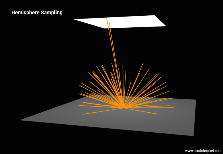
If you examine the figure above, note that of the 64 rays cast, only 2 intersect with the surface of the area light, which is a rather poor ratio. This should hint at the problem with this approach—noise. We are going to need a substantial number of rays to ensure we not only detect the area light but also have enough samples intersecting its surface to properly account for its contribution to the illumination at \(x\).

Here is the pseudocode for the hemisphere sampling method, used to approximate the result of the rendering equation:

uint32_t num_samples = 64;
Vec3f L = 0;
for (uint32_t n = 0; n < num_samples; ++n) {
    // Pick a random direction
    Vec3f rand_dir = ...;
    if (Intersect(x, rand_dir, scene, &isect_info)) {
        if (isect_info.mesh->emission_ != 0)
			// emission_ set to 1 for now (see comment below)
            L += 1 / M_PI * isect_info.mesh->emission_ * max(0, rand_dir.Dot(isect_info.N)) / pdf; 
    }
}
L /= num_samples;

Note the 1/M_PI term, which accounts for the diffuse BRDF. The 1 in the numerator represents \( R(x) \) or the surface albedo. In this case, our ground plane is depicted as pure white—an albedo that doesn't exist in real-life, but this is not a problem for this demonstration. Again, don't worry for now about how we generate these random directions. Let's just say all directions have an equal chance to be chosen among possible directions. Also, don't worry about the division by the pdf variable; we will address this later. So as you can see, we cast 64 rays in this example, whose directions are all contained within the hemisphere of direction along the normal at \(x\). If a ray intersects an emissive mesh (an area light?), then we sum its contribution weighted by the diffuse BRDF and the Lambert cosine law (the dot product between the surface normal and the light direction—which is the sample for which we've chosen a random direction).

As pointed out before, the problem with this approach is that only a few samples are likely to hit the area lights, which is problematic because it produces considerable noise in the image. We can increase the number of rays, but the larger the number, the slower the render time. So, what if we could decrease that noise while keeping the number of samples constant?

We can achieve this goal by inverting the problem. Instead of sampling the hemisphere, we will in turn sample the surface of the area light. Rather than generating random directions within the hemisphere oriented along the normal, we are going to generate samples across the surface of the area light, as shown in the figure below (the method consists of choosing random positions uniformly distributed across the surface of the light. We can then connect each one of these sample points to \(x\) to determine a light direction for each sample. Keep in mind that these \(\omega\) light sample vectors are going from \(x\) to the sample position on the light, which is the reverse order of how light actually travels—from the light to \(x\)).

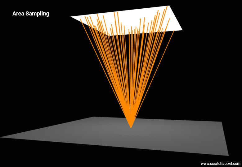
Now, doing this is perfectly acceptable as long as we adjust the mathematics a bit because we need to find a conversion or a relation, should I say, between the surface of the light and how this surface can be expressed in terms of solid angle. What you could do is project the area light onto the hemisphere and sample it there, but it turns out to be a problem that's not straightforward to solve because a polygon projected onto a sphere turns into a spherical polygon for which we have no straightforward representation (as shown in the figure below).

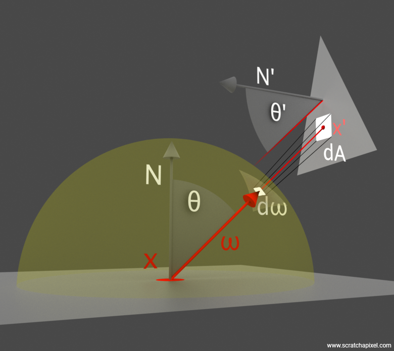
So, what shall we do instead? You can consider each sample on the area light as a small differential area \(dA\) on the surface of the light. What we need to do is somehow "convert" this differential area \(dA\) into a differential solid angle \(d\omega\). Fortunately, the relationship between the two exists and is rather simple:

• where \(\theta'\), or \(\cos^{-1}(-\omega \cdot N')\), is the angle between the light normal \(N'\) and the sample light direction \(\omega\)

• \(x'\) is the sample on the surface of the area light

• \(x\) is the shaded point

• \(|x - x'|\) is the distance from \(x\) to \(x'\)

• \(\omega\), the vector \(\vec{x' - x}\), is the sample light direction

Note that the squared distance in the denominator accounts for the inverse square law, which we introduced in the previous chapter. This physical law arises because light radiates from a source and spreads out spherically. Here, we consider that light is emitted by the area light at \(x'\) both radially and isotropically—that is, uniformly in every direction. Consequently, as explained in the previous chapter, the surface area over which the light spreads increases with the square of the distance from the source.

Our rendering equation now becomes:

The term \(vis(x,x')\) accounts for whether the two points see each other. Note how we now integrate over the area of the light's surface as opposed to over the hemisphere of directions. Wow! Well done. Technically, to turn this into code, we would need to discuss (again) about the probability density function (PDF), but we will get to that in just a moment. For now, trust that the following pseudocode works:

uint32_t num_samples = 64;
Vec3f L = 0;
for (uint32_t n = 0; n < num_samples; ++n) {
    // Pick a random direction on the surface of the light
    Vec3f wi;
	float pdf;
	float t_max;
	Vec3f Le = light->Sample(x, r1, r2, &wi, &pdf, &t_max); 
	if (!Occluded(x, wi, t_max, scene)) // don't look for intersections beyond t_max
		L += 1 / M_PI * Le * max(0, wi.Dot(isect_info.N) * max(0, -wi.Dot(light->normal)) / (t_max * t_max * pdf)); 
}
L /= num_samples;

Note that in the code above, we no longer consider the light as a geometry with emissive properties. It use a light source derived from the Light class. This is why, in most production renderers, area light sources are not visible in the image—they are not treated as geometry by default. More on that soon. Thus, we directly pick the light-emitted energy (Le) from the light, as well as use the light normal, which you will find is super easy to obtain once we delve into the implementation details. t_max, as mentioned before, holds the distance from \(x\) to the sample position \(x'\). The sample position on the surface of the area light is calculated from two random numbers defined in the range [0:1], represented by r1 and r2 in the pseudocode above. More on that will be discussed soon as well. The following figure illustrates the type of image we can achieve with this approach. Further explanations about this probability density function (pdf) will be provided shortly.

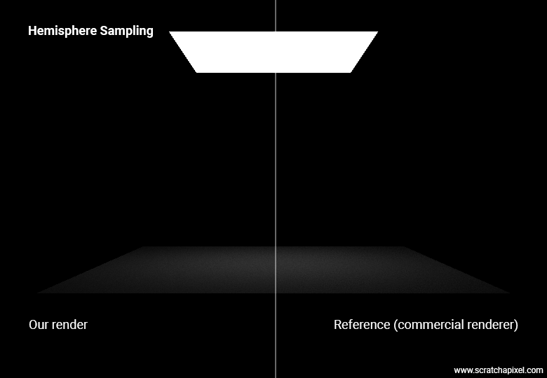
Before we compare the two methods, hemisphere versus area sampling, I want to point out that, as you can see in the image below, the two methods (at least for now) produce a different output.

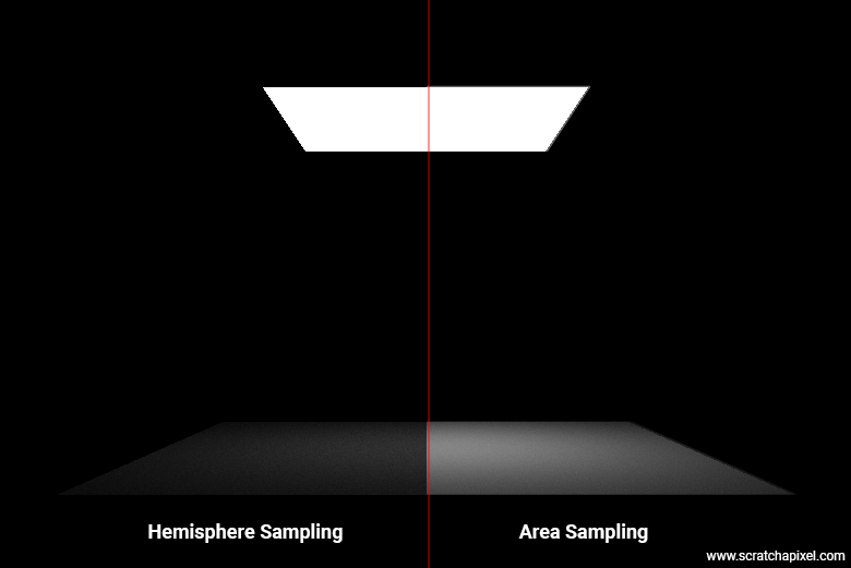
Not good, but it was done on purpose. The image representing the hemisphere sampling method uses an area light whose emission value is (1,1,1)—essentially, 1. Now, in the image that uses the area sampling method, the area of the light is 5.11E+7 square meters (square unit area should I say), its power is 1.34E+8, and therefore its radiant exitance (W/m^2) is 2.62541 W/m^2. If we use this value instead of 1 in the hemisphere sampling method, our images match perfectly.

uint32_t num_samples = 64;
Vec3f L = 0;
for (uint32_t n = 0; n < num_samples; ++n) {
    // Pick a random direction
    Vec3f rand_dir = ...;
    if (Intersect(x, rand_dir, scene, &isect_info)) {
        if (isect_info.mesh->emission_ != 0)
			// emission_ set to 2.62541
            L += 1 / M_PI * isect_info.mesh->emission_ * max(0, rand_dir.Dot(isect_info.N)) / pdf; 
    }
}
L /= num_samples;

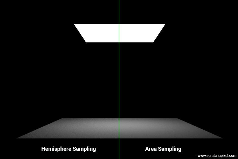
In hemisphere sampling, you are considering how much light energy per square meter is emanating from the surface in a particular direction back towards the point of interest \(x\). Essentially, the hemisphere method leverages statistical sampling to convert the radiometric properties of the light (energy per unit area) into a form that can be integrated over a solid angle. This method transforms an area-based measurement (light source surface area) into an angle-based measurement (solid angle). Therefore, one needs to take care to use the correct "emission" (radiant exitance) value for the geometry when dealing with the hemisphere sampling method, which you can calculate from the area light's power and area as shown above. Alternatively, you can calculate the power of the light based on its known radiant exitance and area if your goal is for the two methods to produce comparable results.

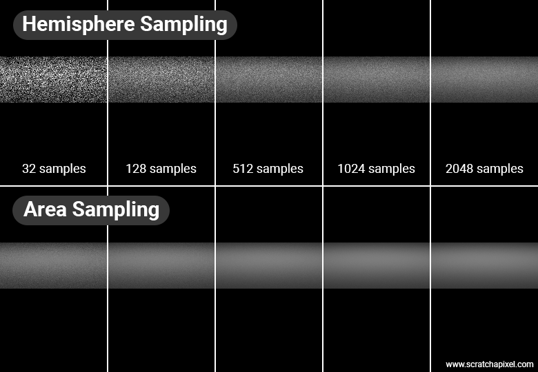
Good. Now our two methods produce the same result. But why have we gone through all this pain already? If you look at the following figure, you can see that for an equal number of samples, the area method produces images with far less noise compared to their hemisphere sampling method counterpart—I mean, significantly less. So, of course, the area method is the one we use for simulating area lights in 3D rendering.

Before we conclude this chapter and look at the C++ code, we need to finally address the topic of the probability density function or pdf variable that we have been referring to in the pseudocode above and have constantly mentioned that you shouldn't worry about it as we will explain it later. Now is the time.

Be ready to raise the difficulty a notch even further.

Introduction to Probability Density Functions (PDF), Probability Distributions and Monte Carlo Estimators

Before we proceed, it's important to clarify a key concept related to the Monte Carlo estimation technique. This is particularly crucial since this isn't primarily a lesson on Monte Carlo methods, and you may not have read the two dedicated lessons yet. The key concept we need to understand is the probability density function (pdf), which we've encountered in the Sample() method for lighting.

We will use a couple of examples to gain an intuition about what the probability density function is and what problem it solves within the context of Monte Carlo integration. Consider the problem by reflecting on what happens when you use the area sampling method for a light that is 1x1 unit in size (that is, it has an area of 1 unit). Suppose you decide to use 16 samples, so you generate your 16 samples across the surface of the light, then calculate the light direction for each sample using the code provided above. Great. But now, let's say you want to sample an area light that is 2x2 units, which is 4 times the area of the initial light. Would you agree that the light, being larger, should have a more significant contribution? Think of it not as the initial light having a larger surface, but as four of the initial lights being packed together to form a larger light. We now have 4 times the amount of energy that the initial light had! Right?

However, if you apply the code we provided for sampling the light (using the area-sampling method), you'll find that there is nothing in the code that accounts for the size of the light. Thus, sampling these two lights would effectively yield the same result, unless you adjust the pdf (probability density function) value for each calculation. This adjustment would ensure that when sampling the larger light, the result would be proportionally larger as well. Imagine the pdf is 1 for the 1x1 size light and 0.25 for the 2x2 size light. Therefore, in the case of the larger light (2x2), the result would be 4 times that of the initial sampling, since we would divide the result of the light contribution by 0.25. It seems we're on the right track!

uint32_t num_samples = 64;
Vec3f L = 0;
for (uint32_t n = 0; n < num_samples; ++n) {
    // Pick a random direction
    Vec3f rand_dir = ...;
    if (Intersect(x, rand_dir, scene, &isect_info)) {
        if (isect_info.mesh->emission_ != 0)
            L += 1 / M_PI * isect_info.mesh->emission_ * max(0, rand_dir.Dot(isect_info.N)) / pdf; 
    }
}
L /= num_samples;

Somehow, the PDF serves as the adjustment variable that we use to account for the relationship between the size of the light and the energy it emits. The larger the light, the smaller the PDF, and consequently, the greater the result of the Monte Carlo approximation. In the case of uniform sampling, the PDF is \(1/\text{Area}\). We will provide more background about the PDF in general and explain more precisely why this PDF (\(1/\text{Area}\)) is effective in this context.

In statistics, you might want to know the probability of a die landing on the number 5. Since the die has six faces, there are only six possible outcomes. Assuming the die is not rigged, there's an equal probability for any of these numbers to be drawn when you throw the die; that probability is \(1/6\). Note that in the case of a die, because we have a limited number of outcomes (6), we say that these probabilities are discrete. Now, what is the probability of a point on the surface of the area light being chosen? The problem is quite different in this case because we no longer deal with discrete outcomes but with a continuous domain (the area light surface represents a continuous range of outcomes). You can choose any value along the x-axis and any value along the z-axis of the light.

What matters here is the term density. In the context of a continuous domain (we spoke about a 2D surface, that of the area light, but it could be a 1D line like a string or a 3D volume), \(p(x)\), where \(p\) here is a probability density function, wouldn't give the probability of occurrence at that point but rather a measure of how dense the probability is distributed around that point. As with any probabilities, the sum of all probabilities must be 1. This is also true of the PDF, but since it is a function, we need to replace the summation (like adding six times \(1/6\), which is the probability of getting any of the numbers on the face of a die) with an integral, so: \(\int p(x) = 1.\), where \(p(x)\) here is our probability density function (it is a function as standard as any function can be in mathematics). The integral of the PDF across the entire surface measures the total probability of drawing a sample from anywhere on the surface, which must logically be 100% (or a probability of 1) because every sample drawn will definitely be from somewhere on that surface. When the emission from the surface is uniform, meaning every part of the surface is equally likely to emit light (or be sampled in the context of Monte Carlo simulations), the PDF must reflect this uniformity. If the surface has an area \(A\), then setting the PDF to \(\frac{1}{A}\) ensures that the probability density is spread evenly across the entire surface. This setting of the PDF ensures that the integral over the surface will sum to one:

By defining the PDF as \(\frac{1}{\text{Area}}\) for a uniformly emitting or sampled surface, the mathematical framework ensures that the probability of selecting any specific portion of that area correctly reflects its relative size to the whole area. This is crucial for accurate, unbiased Monte Carlo simulations, where each part of the sampled domain (like the surface of a light) must have a probability weighted proportionally to its size.

This leads us to the equation of the Monte Carlo estimator—an important term for you to remember, that you will see in every textbook referring to the Monte Carlo method:

This equation shows how the Monte Carlo estimator on the right provides an approximation of the integral of the function \(f(x)\). Here’s what it involves:

• The Monte Carlo estimator consists of an average of the sum of the function \(f(x)\) evaluated at various sample positions \(x_i\), which have been drawn according to the sample distribution \(p\), divided by the probability density function at \(x_i\).

• The term \(x_i \sim p\) indicates that the samples \(x_i\) are drawn from some probability distribution \(p\) (that can be uniform or non-uniform).

Note also that the symbol \(\approx\) denotes approximation. What the Monte Carlo estimator provides is an approximation of \(\int f(x) \, dx\).

In this lesson, thankfully, we will only deal with uniformly distributed samples. I say "thankfully" because the mathematics behind understanding non-uniform distributions is not overly complex, but it does require careful explanation. Please refer to the lesson on Importance Sampling after reading this one if you want to delve further into this topic. The key takeaway from this lesson is that most advanced ray-tracing-based rendering engines rely heavily on Monte Carlo estimators in some shape or form. As we progress, we will learn many more details about this, but the Monte Carlo estimator alone is the fundamental building block upon which most, if not all, of these systems are built.

Applied to our rendering equation when dealing with solid angles (hemisphere sampling approach), we get:

And if we sample the area light (area sampling approach), we can write:

Where:

• \(\theta\) accounts for the angle between the light direction \(\omega\) and the surface normal at \(x\).

• \(\theta'\) is the angle between the light normal at \(x'\) and the light direction.

• \(x\) is the shaded point on the object's surface.

• \(x'\) is a sample on the surface of the light (sampled from the probability distribution \(p(x)\)).

• \(p(x)\) is our probability distribution function (which should be \(1/\text{Area}\) in the case of uniformly distributed samples).

• \(r\) is the distance from \(x\) to \(x'\).

• \(\text{vis}(x,x')\) is a function that returns 1 if the two points are visible to each other, 0 otherwise.

We have omitted the BRDF for diffuse surfaces from the summation since it's a constant.

Before we move to the next chapter and provide you with the actual implementation of this technique for various canonical shapes of area lights, it might be useful to break down how you should apply the equation above in practice. As illustrated in this equation:

There are two parts:

• The first part, \(\frac{1}{N} \sum_{i=1}^N \frac{f(x_i)}{p(x_i)}\), is the Monte Carlo estimator.

• The second part, \(x_i \sim p\), is where you start when implementing this algorithm in code. Technically, it involves drawing a random variable \(x_i\) according to the probability distribution \(p\).

Currently, we only deal with a uniform distribution, so the PDF is constant (1/Area) as already mentioned several times. However, this is not always the case. For example, imagine a rectangular area light mapped with a texture of a disk that is super bright in the center and fades out at the edges. Intuitively, it would make sense to generate more samples where the texture is brightest, which is where the light contributes most in terms of energy to the illumination of the scene. This approach would be more effective than uniform sampling, which treats areas of high and low light contribution equally.

The figure below (Figure 17) compares a uniform versus a non-uniform sampling strategy. On the left, the surface of the rectangular area light was sampled using a uniform distribution. Note that many samples fall in the darker regions of the light, even though these samples contribute very little to the overall light contribution, since most of the light energy is concentrated towards the center of the light. On the right, the samples were drawn according to a probability distribution that gives more importance to areas of the light where there is more energy, thus more towards the center than towards the edges. It should be noted that in the left image, the PDF of each sample is constant and equal to 1/Area. On the right, each sample has its own PDF values, with higher values where the samples are most concentrated and lower values where samples are sparse, reflecting the uneven distribution in the summation of the Monte Carlo estimator.

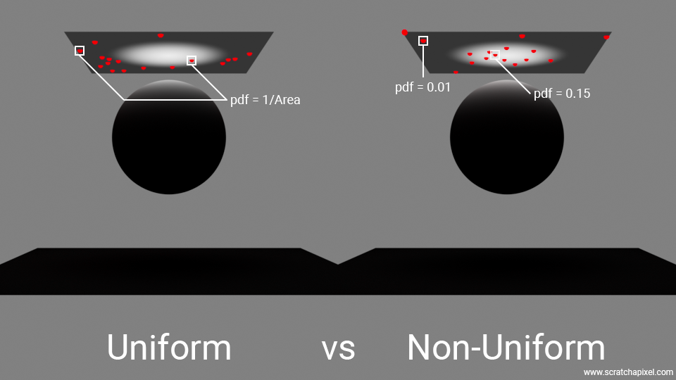
With this approach, we would draw samples from a probability distribution function that generates more samples in the center of the area light than on the edges. As a result of this uneven distribution of samples, we would need to adjust the PDF value accordingly, where samples in the center, because they are more concentrated, would have a higher PDF than those at the edges. Intuitively, this makes sense: if there is a higher probability of generating a sample where the light is brightest (due to the texture applied), of course, the PDF would be larger. But remember, the PDF is used in the denominator of the MC estimator. Thus, the higher the denominator, the smaller the result of the division. In other words, samples that are more likely to be produced—typically from the brighter areas of the texture—contribute less to the overall approximation due to their higher PDF values. Conversely, samples from darker regions of the texture, which are less likely to be produced, contribute more due to their lower PDF values. This may seem counterintuitive, but it's a strategic balance: since there are more samples from the high-probability (bright) areas, the division by the PDF effectively equalizes the contribution across the light's surface. This approach ensures that the uneven distribution of samples, dictated by varying light intensity across the texture, does not skew the overall lighting estimation. By using the PDF in the denominator of the Monte Carlo estimator, we precisely compensate for this uneven sample distribution, allowing for a more accurate representation of the light's actual impact on the scene.

This concept is fundamental in the use of the Monte Carlo method. It ensures that while choosing samples from a probability distribution that is not necessarily uniform, the approximation does not become skewed or biased towards the samples that are more likely to be drawn due to that non-uniform sample distribution. Utilizing a non-uniform PDF has the considerable advantage of selecting areas in the integration domain that are more likely to have a high contribution to the approximation than others with lesser contributions, effectively allowing us to reduce variance (which translates to noise reduction for us).

But this is not the focus for now. The reason why we've delved into this explanation is primarily to understand the initial steps of implementing the Monte Carlo method, which involves generating samples according to a specific probability distribution function. Through these examples, you have hopefully developed an intuitive understanding of how this works. Don't worry; in the next chapter, we will explore a couple of practical examples with code.

So, in summary, this is how you should read this equation and implement it in practice:

• Generate Samples According to a PDF: If the area light features a texture with a bright spot in the middle, we aim to generate more samples where the texture has high values because these are the areas of the light that contribute the most to the approximation of light contribution (this method is a variance reduction technique that we will learn more about later in this lesson and in subsequent lessons devoted to sampling techniques. Another term used for this method is importance sampling). That’s what it means when one says "draw samples according to a given PDF or a given distribution". However, for now, we will use a uniform distribution, which, as we have learned above for rectangular lights, is \(1/\text{Area}\). In some textbooks, this step is referred to as the sampling procedure (sometimes denoted \(Sp\)). We will explore such methods in the next chapter—they encapsulate the logic for generating these samples whose distribution matches that of the chosen PDF.

• Use the Drawn Samples in Your Monte Carlo Estimator: Once we have drawn the samples from the PDF and determined the probability of those samples (our \(x'\)s) from the PDF itself, we can use these samples to evaluate the function \(L_e(x')\), divide \(L_e(x')\) by \(p(x')\) (the probability of \(x'\)), and add the result to our summation. This total is then divided by the number of samples once all the samples have been processed.

Returning to our initial example, the light is 1x1 in size, so the PDF (which is constant for now, as we've only discussed uniform distribution) is 1. When the light is 2x2 in size, the PDF becomes \(1/4\). Effectively, dividing the \(L_e\) at these sample positions by 0.25 means the contribution of the light is four times greater than that of the 1x1 light.

This corresponds to the code we have been using for the area sampling method, in which the pdf was effectively set to \(1/\text{Area}\). Although we don't show in this code how the area is calculated, we will provide the full source code for that in the next chapter.

uint32_t num_samples = 64;
Vec3f L = 0;
for (uint32_t n = 0; n < num_samples; ++n) {
    Vec3f wi;
    float pdf;
    float t_max;
    Vec3f Le = light->Sample(x, r1, r2, &wi, &pdf, &t_max); 
    if (!Occluded(x, wi, t_max, scene)) // don't look for intersections beyond t_max
        L += 1 / M_PI * Le * max(0, wi.Dot(isect_info.N) * max(0, -wi.Dot(light->normal)) / (t_max * t_max * pdf)); 
}
L /= num_samples;

In the pseudocode above, t_max accounts for \(r\) and pdf accounts for \(p(x)\). Note that as \(\omega_i\) goes from \(x\) to \(x'\), we need to invert the dot product between the light sample and the light normal in -wi.Dot(light->normal).

Sampling Strategies

Before we conclude this chapter (haven’t I mentioned that a few times already?), I want to highlight an important aspect related to the generation of these samples. So far, even though we haven’t explored the code and thus don’t know how these samples are generated, we've been showing examples where the samples are randomly distributed. However, as you can observe in the produced pictures, notably Figure 17 (left), this "naive" approach may produce clusters of samples. The random nature of sample generation makes it unpredictable whether clusters—bunches of samples close to each other—will form. This clustering is problematic because it results in many samples in the same region of the light, leaving other areas under-sampled.

What I want to emphasize here is that there are much better methods for generating these samples—beyond the importance sampling method we've touched upon in this chapter. A significant portion of the literature is devoted to designing algorithms that generate the best possible sampling patterns, methods that avoid creating these clusters while maintaining their inherent random property, which is essential for the Monte Carlo method to work.

As this is a topic extensive enough to merit several dedicated lessons, we won't delve deeper into it now, but I wanted you to be aware of this. If you are specifically interested in this topic, check out our lessons on Sampling Strategies and Importance Sampling.

Practical Implementation Details

We had to divide this part of the lesson into two chapters because understanding how to implement area lights requires some theoretical or mathematical tools that we have quickly and hopefully intuitively and gently introduced you to in this chapter. But we understand your frustration if you feel you don't yet fully grasp the complete picture for implementing these area lights. This will be the topic of the next chapter, in which we will provide you with the code and look at the gritty details for implementing 4 types of area lights:

• Rectangular

• Spherical

• Disk

• Triangular

In the next chapter, we will also provide references at the end to the papers that introduced most of these techniques.

There will be a bit more theory in the next chapter as we will need to consider non-uniform sampling and other sampling methods, namely angular sampling, which is the counterpart of area sampling but for angles rather than surfaces. Congratulations if you've made it this far! We believe you have been exposed to some of the best educational material on the topic, and hopefully, we have saved you years of feeling that you are navigating in the dark. If you liked this content, please support our work and consider making a donation.