Spherical Area Light: Using Cone Sampling
Reading time: 42 mins.Preamble
Because each shape that an area light can have has its own specific implementation considerations, we have decided to dedicate one page per area light shape. More specifically, we will consider triangular, planar, disk, and finally spherical area lights. This preamble is repeated on each page to ensure that if you landed on one of these pages from an external link, you are aware that it is advisable to start by reading the page on the triangular area light. There, we will discuss some concepts that will be reused across the other light types and provide a general explanation about the code we will be using to implement these lights.
Also note that we strongly recommend that you read the lessons on Distributed Ray-Tracing and Stochastic Sampling and Sampling Strategies, which are corollaries to this one.
Cone/Angle Sampling
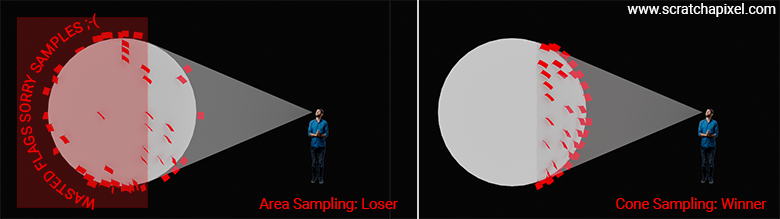
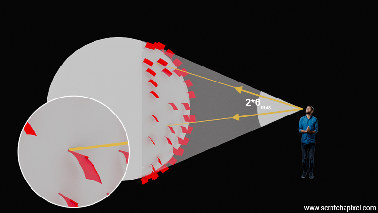
As suggested in the previous chapter, in which we showed how to implement the area sampling method to uniformly sample a sphere, the area sampling method is perfectly valid. However, it has a drawback in that samples generated at the back of the sphere, as seen from the shaded point \(x\), are "wasted" (they don't contribute to the illumination of the shaded point since they point away from it). If you look at the scene in which we have a shaded point \(x\) and a sphere acting as an area light, you can see that all samples visible from \(x\) are contained within a cone. Since we are looking for an alternative to sampling the surface of the sphere, why not just select directions from within that cone of directions? Indeed, if we trace rays in those directions (not quite literally, as we will soon show), each one of these directions should correspond to a point on the sphere, and each one of these samples should be effectively visible from \(x\). That's what we want. So the question now is: is it possible to uniformly sample directions within that cone? It happens that the answer is yes, and this is what we will study in this chapter.
Note that this method is exactly similar to sampling the hemisphere, which we studied in the chapter Area Lights: Mathematical Foundations. We know this method is also valid for evaluating the contribution of area lights. The key difference is that in the cone sampling case, we constrain the generation of sample directions to the solid angle subtended by the spherical area light, whereas in the hemisphere sampling method, we sample the entire hemisphere of directions.
In the former case (cone sampling), each generated sample should correspond to a point on the spherical light. In the latter (hemispherical sampling), we don't know if any given generated samples will hit an area light or not.
But before we delve into the math, a little bit of history. In the literature, you might see this technique under different names. In the paper in which it was first introduced (let us know if you know of an earlier resource), "Monte Carlo Techniques for Direct Lighting Calculations" by Peter Shirley and Changyaw Wang (1996), it's referred to as sampling uniformly in directional space. However, you will also see it being called cone sampling because in this particular case (sampling a sphere), the shape is a cone. But if you consider the more general case (say you want to sample a triangle using this technique, which is possible as mentioned in the chapter devoted to sampling triangular light, a technique that we will study in a future revision of this lesson), it is better to speak of angle sampling (or solid angle sampling). While quite seminal, I have to say that "Monte Carlo Techniques for Direct Lighting Calculations" is typical of one of those papers that is quite hard to read if you don't have a solid background in mathematics and a mind capable of juggling abstract concepts. Well, that's how things used to be in the good old days and one of the reasons that pushed us to create Scratchapixel. We think we can, or more precisely that we should, do much better.
Now that we've covered that, let's delve into the mathematics. The process we will follow can be divided into two steps:
-
Step 1: Initially, we need to learn how to generate uniformly distributed sample directions within the cone subtended by the spherical area lights. These are directions.
-
Step 2: Each direction generated in Step 1 corresponds to a specific point on the surface of the sphere. Therefore, we need to determine the position on the sphere's surface based on the direction generated. As you will soon discover, this task is not as straightforward as one might assume.
Step 1: Generating Uniformly Distributed Sample Directions within the Cone Subtended by the Spherical Light
First, the cone we are talking about, as depicted in the following figure, is the one you can draw by connecting (in 2D) the shaded point \(x\), forming the apex of the cone, to the points where the lines starting from \(x\) and tangent to the surface of the sphere intersect the sphere. As you can see in the following figure, the half-angle \(\theta\) is the angle subtended by the cone's base (divided by 2).
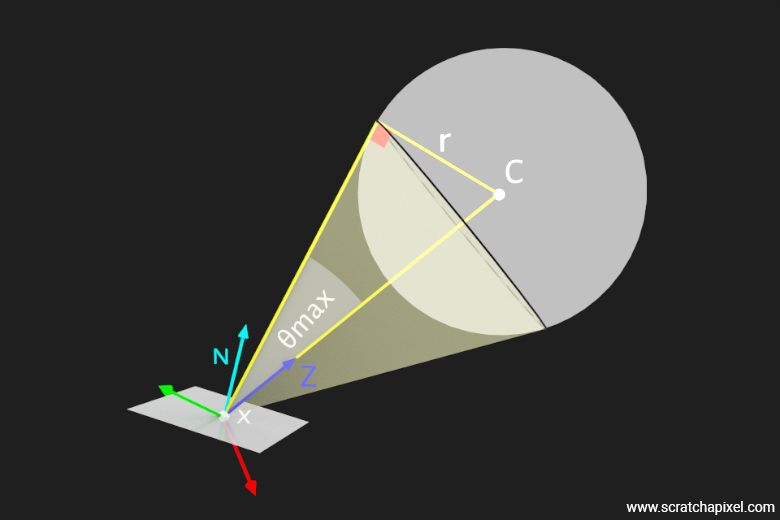
It is quite simple to calculate that angle. We know the distance from \(x\) to the sphere center, and we know the sphere radius. By construction, as shown in the figure, if we consider a line starting from the sphere center \(C\), and intersecting the lines tangent to the sphere such that these two lines form a right angle, we can use the trigonometric ratio \(\sin(\theta) = \frac{\text{opposite side}}{\text{hypotenuse}}\) to find the value of that angle. We will call this angle \(\theta_{\text{max}}\) because it is the maximum (polar) angle any of our sample directions may have within that cone. (Don't worry too much if the reason we mentioned "polar" here doesn't make sense to you yet - we will explain that shortly.)
$$ \sin(\theta_{\text{max}}) = \dfrac{r}{||c - x||} $$The following video will help you visualize the setup and its various parts (hopefully) with a 3D representation.
In the video, we rotated the whole setup so that the Z vector, pointing from the shaded point \( x \) to the sphere center \( C \), points upward. When we generate samples using the spherical to Cartesian coordinates equations, the resulting vector coordinates are defined within the Cartesian coordinate system of the unit sphere, where the Z-axis has coordinates (0, 1, 0). Once generated in this coordinate system (that of the unit sphere, more precisely the cone subtended by the sphere, where the cone axis is aligned with the vector (0, 1, 0)), we will need to rotate the sample directions back so they ultimately align with the Z-axis pointing from the shaded point to \( C \), the sphere's center. Later in this lesson, we will show how to perform that rotation. In the video, we also mentioned that we will be using the name z-vector to denote the up vector here rather than the y-vector, which we've typically used so far. No panic, this is not a mistake.
It just happens that when you get into the shading world, people tend to prefer a convention in which the Z vector denotes the up vector, while the X (1, 0, 0) and Y (0, 0, 1) axes are the tangent and bitangent of that vector, respectively. Considering this is the convention you will see used in almost all papers devoted to shading, it's better for us to stick to it as well.
We will now consider \( \phi \) as our azimuthal angle, ranging from 0 to \( 2\pi \), and \( \theta \) as our polar angle. Note that in the context of a sphere, the polar angle typically ranges from 0 to \( \pi \). However, for our purposes, we only need to sample a subspace of the sphere covered by our solid angle, which means \( \theta \) will vary from 0 to \( \theta_{\text{max}} \).
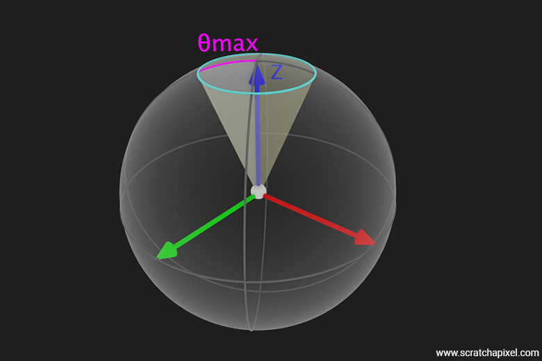
If you observe the figure above, \( \phi \) defines a position on the circle centered around the z-axis, with a radius defined by \( \theta \). This method allows us to cover every possible direction within the solid angle subtended by the spherical light.
From a convention standpoint, we are returning to the conventions used in the previous chapter for the theoretical part. This is the convention commonly used by physicists, where the z-axis is considered the up vector, and the Cartesian coordinate system typically uses a left-hand coordinate system. However, we will define \(\theta\) and \(\phi\) as the polar and azimuthal angles, respectively, as typically used by physicists. In the previous chapter, we used \(\phi\) and \(\theta\) as the polar and azimuthal angles, which are the conventions preferred by mathematicians.
Let's state our objective: Our objective is to use two random uniformly distributed numbers in the range 0 to 1 to generate a sample direction with spherical coordinates \(\theta\) and \(\phi\) with respect to the Cartesian coordinate system we just defined. This ensures that the resulting directions (once converted from spherical coordinates to Cartesian coordinates) are uniformly distributed within the cone subtended by the sphere. Once we have these directions, we will see how we can calculate the sample positions on the sphere from these directions (though we will see that we won't necessarily need to convert the directions from spherical to Cartesian coordinates to do so, but more on that later). So first things first: how do we sample \(\theta\) and \(\phi\) to generate these uniformly sampled directions within the cone?
Note that the problem we are trying to solve is very similar to that of sampling the sphere area uniformly. The first step is to calculate the solid angle of the cone subtended by the sphere. Remember that the solid angle \(\Omega\) subtended by a surface is given by:
$$ \Omega = \int_{\text{surface}} \sin(\theta) \, d\theta \, d\phi. $$We touched on this equation in the previous chapter when we mentioned that the differential area \(dA\) for a sphere of radius \(r\) is equal to \(r^2 \sin(\theta) \, d\theta \, d\phi\). Here, we are dealing with a unit sphere, so \(r = 1\). In this context, \(\theta\) is the polar angle (measured from the z-axis), and \(\phi\) is the azimuthal angle (measured in the x-y plane). For a cone with a half-angle \(\theta_{\text{max}}\), the azimuthal angle \(\phi\) ranges from 0 to \(2\pi\) and the polar angle \(\theta\) ranges from 0 to \(\theta_{\text{max}}\). The solid angle \(\Omega\) subtended by this cone is:
$$ \Omega = \int_0^{2\pi} \int_0^{\theta_{\text{max}}} \sin(\theta) \, d\theta \, d\phi $$Integrating with respect to \(\theta\) gives:
$$ \int_0^{\theta_{\text{max}}} \sin(\theta) \, d\theta $$The integral of \(\sin(\theta)\) is \(-\cos(\theta)\):
$$ \left[ -\cos(\theta) \right]_0^{\theta_{\text{max}}} = -\cos(\theta_{\text{max}}) - (-\cos(0)) = -\cos(\theta_{\text{max}}) + 1 $$Simplifying:
$$ 1 - \cos(\theta_{\text{max}}) $$Integrating with respect to \(\phi\):
$$ \int_0^{2\pi} d\phi = 2\pi $$Combining the results:
$$ \Omega = 2\pi (1 - \cos(\theta_{\text{max}})) $$You can find another proof for the solid angle equation in the paper Solid Angle of Conical Surfaces, Polyhedral Cones, and Intersecting Spherical Caps by Oleg Mazonka (2012). However, be warned that this demonstration is rather involved mathematically. As this is an introductory lesson, we will not go through that proof here. Hopefully, there will be time in the future to create a much more accessible version of this paper.
As we know, the PDF of a random variable uniformly distributed (with respect to the solid angle in our case, but this is similar to area) within the cone is the reciprocal of the solid angle subtended by the cone. Therefore:
$$ \text{Uniform density} = \frac{1}{\Omega} = \frac{1}{2\pi (1 - \cos(\theta_{\text{max}}))} $$This would effectively be the PDF (let's call it \(p(\omega')\)) for sampling directions uniformly within the cone defined by \(\theta_{\text{max}}\). Here, \(\omega'\) represents the solid angle, and this PDF accounts for both the azimuthal \(\phi\) and the polar angle \(\theta\). Now, similarly to the way we've sampled the azimuthal angle for the sphere area-sampling method, we can observe that given the symmetry around the z-axis, the azimuthal angle \(\phi\) is uniformly distributed from 0 to \(2\pi\). The PDF for \(\phi\) is thus:
$$ p(\phi) = \dfrac{1}{2\pi} $$Next, we need to find the PDF for \(\theta\). To find the PDF for \(\theta\), we first note that the PDF given above represents a uniform distribution over the solid angle. For the polar angle \(\theta\), we typically use \(\cos(\theta)\) because it simplifies the calculations due to the trigonometric nature of the sphere. To sample \(\theta\) uniformly within the cone, we first consider the range of \(\cos(\theta)\):
-
When \(\theta = 0\), \(\cos(0) = 1\)
-
When \(\theta = \theta_{\text{max}}\), \(\cos(\theta_{\text{max}})\)
Thus, \(\cos(\theta)\) ranges from \(\cos(\theta_{\text{max}})\) to 1. For a uniform distribution over this range, the PDF for \(\cos(\theta)\) is given by:
$$ p(\cos(\theta)) = \frac{1}{1 - \cos(\theta_{\text{max}})} $$For a uniform distribution of a random variable \(X\) over an interval \([a, b]\), the PDF \(p(X)\) is given by:
$$ p(X) = \dfrac{1}{b - a} $$Since the range of \(\cos(\theta)\) is \([\cos(\theta_{\text{max}}), 1]\), the length of the interval is \([1 - \cos(\theta_{\text{max}})]\), and so the PDF we are looking for is:
$$ p(\cos(\theta)) = \dfrac{1}{1 - \cos(\theta_{\text{max}})} $$To find the PDF for \(\theta\) from the PDF of \(\cos(\theta)\), we apply the change of variables formula. If \(u = \cos(\theta)\), then \(du = -\sin(\theta) \, d\theta\). The PDF transformation is given by:
$$ p(\theta) = p(\cos(\theta)) \left| \frac{d(\cos(\theta))}{d\theta} \right| $$Since \( \frac{d(\cos(\theta))}{d\theta} = -\sin(\theta) \):
$$ p(\theta) = \frac{1}{1 - \cos(\theta_{\text{max}})} \left| -\sin(\theta) \right| = \frac{\sin(\theta)}{1 - \cos(\theta_{\text{max}})} $$Here is the key idea behind the change of variables formula. When you have a random variable \(X\) with a PDF \(p_X(x)\), and you define a new random variable \(Y = g(X)\), the PDF \(p_Y(y)\) of the new random variable \(Y\) can be found using the formula:
$$ p_Y(y) = p_X(x) \left| \frac{dx}{dy} \right| $$where \(x = g^{-1}(y)\) and \(\left| \frac{dx}{dy} \right|\) is the absolute value of the derivative of \(x\) with respect to \(y\).
If you want to learn more about this method, which is crucial for understanding concepts such as cone sampling (without it, you might get stuck looking at the final result without ever understanding how to get there), search for "transformation of PDFs," "transformations of random variables," or "change of variables for PDFs."
In conclusion, we have:
-
PDF for \(\phi\):
$$ p(\phi) = \frac{1}{2\pi} $$ -
PDF for \(\theta\):
$$ p(\theta) = \frac{\sin(\theta)}{1 - \cos(\theta_{\text{max}})} $$
That covers the first step in the process of uniformly sampling our cone, which is to find a CDF for it. The next step, as explained in the previous chapter where we used this method to derive a solution for sampling the sphere using the area method, is to calculate a CDF from the PDF. Remember that to do so, we need to integrate the PDF from the lower bound of the integration domain, which in this case is \(0\) to \(\theta\), the integrated random variable. Let's do that. The CDF of \(\theta\) is:
$$ \begin{aligned} F(\theta) &= \int_{0}^{\theta} p(\theta') \, d\theta' \\ F(\theta) &= \int_{0}^{\theta} \frac{\sin(\theta')}{1 - \cos(\theta_{\text{max}})} \, d\theta' \end{aligned} $$Let's now evaluate this integral, starting by moving the constant part to the left of the integral:
$$ \begin{aligned} F(\theta) &= \frac{1}{1 - \cos(\theta_{\text{max}})} \int_{0}^{\theta} \sin(\theta') \, d\theta' \\ F(\theta) &= \frac{1}{1 - \cos(\theta_{\text{max}})} \left[ -\cos(\theta') \right]_{0}^{\theta} \\ F(\theta) &= \frac{1}{1 - \cos(\theta_{\text{max}})} \left( -\cos(\theta) + \cos(0) \right) \\ F(\theta) &= \frac{1}{1 - \cos(\theta_{\text{max}})} \left( 1 - \cos(\theta) \right) \end{aligned} $$That's it, we now have the CDF. The cumulative distribution function, if you remember from the previous chapter, represents the probability that the angle \(\theta\) you chose at random (anything between 0 and \(\theta_{\text{max}}\)) is lower than that random variable \(\theta\). Again, think of it this way: pick a random number between 1 and 6 and ask yourself what's the probability that if I throw a dice on the table, the resulting number will be equal to or lower than that value that I picked at random. All that's left to do (again, read the previous chapter if you are unaware of this method) is to invert the CDF, which is super easy. To find \(\theta\) from a uniform random variable \(\varepsilon_2\) (uniformly distributed in the range [0,1]):
$$\varepsilon_2 = F(\theta) = \frac{1 - \cos(\theta)}{1 - \cos(\theta_{\text{max}})}$$Solving for \(\cos(\theta)\):
$$\cos(\theta) = 1 - \varepsilon_2 (1 - \cos(\theta_{\text{max}}))$$Finally, solving for \(\theta\):
$$\theta = \arccos\left(1 - \varepsilon_2 (1 - \cos(\theta_{\text{max}}))\right)$$That's it. We separated the PDFs for \(\theta\) and \(\phi\) and derived the necessary inverse CDF to sample \(\theta\) so that the resulting sample direction will be uniformly distributed within the cone subtended by the sphere (the area light).
We now have the two equations required to sample the directions in spherical coordinates \(\theta\) and \(\phi\), respectively. While we've completed the mathematical aspect, there's still a geometric consideration to address. Recall that we previously established a canonical Cartesian coordinate system where the z-axis points straight up, and the x-axis and y-axis lie in the horizontal plane, as depicted in the following figure. We've done this because, when you generate samples using the equations to convert from spherical to Cartesian coordinates, these equations:
$$ \begin{array}{l} x = \cos(\phi) \sin(\theta) \\ y = \sin(\phi) \sin(\theta) \\ z = \cos(\theta) \end{array} $$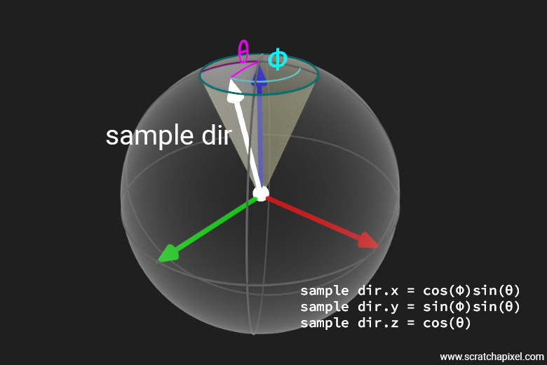
The resulting samples are defined with respect to that coordinate system, which we will call the unit sphere coordinate system for lack of a better name (which I sometimes refer to as the canonical coordinate system to emphasize that I am referring to that of the unit sphere).
However, if you refer to the various figures of the setup we provided so far, you can see that the z-vector is not pointing up but is pointing from the shaded point \(x\) to \(C\), the sphere center.
Remember that in shading, the up vector by convention is the z-axis, not the y-axis.
So, we somehow need to rotate the sample vectors generated within the unit sphere (in our case, limited to the cone, so all sample directions generated within that cone will have their angle \(\theta\) constrained within the range 0 to \(\theta_{\max}\)) so that the coordinate system's z-axis is aligned with the line going from \(x\) to \(C\). We use a small technique here which is quite handy and very often used in shading. We are going to build what we call a local coordinate system (again, here for lack of a better term and to differentiate it from the Cartesian coordinate system of the unit sphere, whose z-axis is up and has coordinates (0,1,0)). Building a local coordinate system from a single vector, such as the vector pointing from \(x\) to \(C\), is described in Creating an Orientation Matrix or Local Coordinate System. Once the samples are generated within the Cartesian coordinate system of the unit sphere (with the z-axis being (0,1,0)), we can rotate them within the local coordinate system using the following code:
Vec3 sample_rotate = sample.x * x + sample.y * y + sample.z * z;
Where x, y, and z here are the x-, y-, and z-axes of the local Cartesian coordinate system, and sample.x, sample.y, and sample.z are the coordinates of the sample direction generated within the unit sphere Cartesian coordinate system.
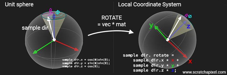
You might wonder why this works and where this equation is coming from, but if you look more closely, you will see that this equation is similar to a vector-matrix multiplication. Indeed, if you consider this equation:
$$ \begin{bmatrix} x' & y' & z' \end{bmatrix} = \begin{bmatrix} x & y & z \end{bmatrix} \begin{bmatrix} \textcolor{red}{a_{11}} & \textcolor{red}{a_{12}} & \textcolor{red}{a_{13}} \\ \textcolor{green}{a_{21}} & \textcolor{green}{a_{22}} & \textcolor{green}{a_{23}} \\ \textcolor{blue}{a_{31}} & \textcolor{blue}{a_{32}} & \textcolor{blue}{a_{33}} \end{bmatrix} $$As you can see in the equation above, we have colored the coefficients so that you can more easily see how they relate to the local coordinate system axes. Now if you expand this equation, you get:
$$ \begin{aligned} x' = x * \textcolor{red}{a_{11}} + y * \textcolor{green}{a_{21}} + z * \textcolor{blue}{a_{31}} \\ y' = x * \textcolor{red}{a_{12}} + y * \textcolor{green}{a_{22}} + z * \textcolor{blue}{a_{32}} \\ z' = x * \textcolor{red}{a_{13}} + y * \textcolor{green}{a_{23}} + z * \textcolor{blue}{a_{33}} \end{aligned} $$This is effectively equivalent to:
$$ v' = x * \textcolor{red}{\text{x-axis}} + y * \textcolor{green}{\text{y-axis}} + z * \textcolor{blue}{\text{z-axis}} $$If you are curious, this technique is also used in the lesson Global Illumination and Path Tracing: A Practical Implementation to rotate samples generated within the hemisphere to a local coordinate system. It will be extensively used in the following lessons devoted to shaders. We won't delve deeply into describing this technique here, as we've directed you to resources where you can learn more about it.
Here is the code snippet used to construct that local coordinate system (aslo sometimes referred to as a the local frame), where v1 (or the z-axis), as shown in the figure, is the normalized vector from the shaded point \(x\) to the sphere's center, and v2 and v3 are the y-axis and x-axis (or tangent and bitangent) of the coordinate system, respectively:
inline void CoordinateSystem(const Vec3f& v1, Vec3f& v2, Vec3f& v3) {
    if (std::fabs(v1.x) > std::fabs(v1.y)) {
        float inv_len = 1 / std::sqrt(v1.x * v1.x + v1.z * v1.z);
        v2 = Vec3f(v1.z * inv_len, 0, -v1.x * inv_len);
    }
    else {
        float inv_len = 1 / std::sqrt(v1.y * v1.y + v1.z * v1.z);
        v2 = Vec3f(0, -v1.z * inv_len, v1.y * inv_len);
    }
    v3 = v1.Cross(v2);
}
There is a paper entitled Building an Orthonormal Basis, Revisited by Tom Duff, James Burgess, Per Christensen, Christophe Hery, Andrew Kensler, Max Liani, and Ryusuke Villemin (yes, all these people), proposing an even better method to calculate an orthonormal basis from a unit vector. While their paper uses a third method for comparison called Frisvad's method, they show that this other method can also fail on some occasions. Therefore, they developed an alternative approach, which is supposed to provide the most reliable way of building such a local coordinate system so far. Who could have thought that such a seemingly trivial problem would cause people to put so much brain power into it? It happens that this is a very critical piece of code that is very often used in ray-tracing, notably when it comes to shading, and that coming up with the most numerically stable solution to this problem is utterly important.
Anyway, here is the code from the paper that we will be using (leaving the first method here for future reference):
inline void CoordinateSystem(const Vec3f& n, Vec3f& b1, Vec3f& b2) {
    float sign = std::copysign(1.0f, n.z);
    const float a = -1.0f / (sign + n.z);
    const float b = n.x * n.y * a;
    b1 = Vec3f(1.0f + sign * n.x * n.x * a, sign * b, -sign * n.x);
    b2 = Vec3f(b, sign + n.y * n.y * a, -n.y);
}
Note that while calling this method will significantly impact computing time, inlining it is probably a good idea, even though we haven't seen any noticeable improvement in doing so. Now that we have this coordinate system, we can proceed to generate the sample directions. To accomplish this, we'll use the UniformSampleCone function, defined as follows:
Vec3f UniformSampleCone(float r1, float r2, float cos_theta_max, const Vec3f& x, const Vec3f& y, const Vec3f& z) {
    float cos_theta = std::lerp(r1, cos_theta_max, 1.f);
    float sin_theta = std::sqrt(1.f - cos_theta * cos_theta);
    float phi = 2 * M_PI * r2;
    return std::cos(phi) * sin_theta * x + std::sin(phi) * sin_theta * y + cos_theta * z;
}
You'll notice the simplification of the equation \(\cos(\theta) = 1 - \varepsilon_2 (1 - \cos(\theta_{\text{max}}))\) to a straightforward std::lerp(r1, cos_theta_max, 1.f). To understand why, consider that treating \(\varepsilon\) as \(1 - \varepsilon\) is equally valid (since they are both random numbers). Thus, if we rewrite the equation as a linear combination \(\cos(\theta) = a \cdot (1 - \varepsilon) + b \cdot \varepsilon\) with \(a = \cos(\theta_{\text{max}})\) and \(b = 1\), and replace \(\varepsilon\) with \(1 - \varepsilon\), we obtain:
In the method UniformSampleCone, the sample direction coordinates x, y, and z, as defined in the Cartesian coordinate system of the unit sphere, are multiplied respectively by the x, y, and z axes of the local coordinate system. This has the effect of rotating the sample from the unit sphere Cartesian coordinate system, where the z-axis has coordinates (0,1,0), into the local Cartesian coordinate system, where the z-axis is pointing from \(x\) to \(C\). The samples are now within the cone of directions subtended by the sphere. The following short video shows this process in action.
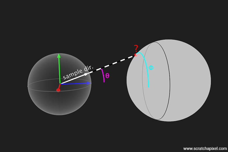
Step 2: Determining the Position on the Spherical Light from the Direction
We know how to generate samples uniformly distributed within the solid angle subtended by the spherical area light. These sample directions point towards the "visible face" of the light (as seen from the shaded point), but what we are interested in is a point on the sphere, not just a direction. So, we will use these directions to find the positions on the surface of the light that these directions point to. Most renderers, when it comes to this part of the algorithm, choose to simply call a ray-sphere intersection routine. That simple. We've studied a couple of methods to do so in the lesson A Minimal Ray-Tracer: Ray-Sphere Intersection, one using a geometric solution and the other using an analytic solution. Both methods are correct, and open-source projects such as PBRT or Mitsuba use the latter.
Though there is a significant difference. The PBRT method assumes that a nonlinear scaling transformation might be applied to the sphere (transforming it into an ellipsoid) and thus requires both the ray origin and direction to be transformed into the sphere's object space before calling the function to find the possible roots of the quadratic form of the sphere. Conversely, the Mitsuba method assumes there's no such non-uniform scaling applied to the sphere and therefore doesn't require the ray direction and origin to be transformed back into the sphere's object space. This second method is better for us because we are not storing the world-to-object matrix for the sphere light anyway and do expect the sphere light to remain a sphere. We will thus use that approach (which still requires transforming the ray origin's position such that the sphere is assumed to be centered at the origin).
Anyway, the code for calculating the intersection between a ray and a sphere using both approaches was already provided in the lesson A Minimal Ray-Tracer: Ray-Sphere Intersection as mentioned earlier, so we won't spend time detailing it here again. What we will do from a code standpoint is add to the Sphere class an Intersect method which returns a boolean indicating whether the ray intersects the sphere or not.
You might think, technically, since all the rays are generated within the solid angle subtended by the sphere, all rays generated within that cone should intersect the sphere. True; however, the problem is that the Intersect routine might return false sometimes for rays that are right at the edge and/or when the spherical light is small and/or the distance to the sphere is large, leading to floating precision errors that result in inaccurate outcomes. That's why writing code can't inherently always lead to 100% expected results.
What most renderers do to fix that problem is to "project" the ray onto the sphere when this happens (hopefully rarely but more often than you may think) because it is assumed that the rays that cause the intersection function to fail are necessarily those that are nearly tangent to the sphere surface, those that touch the sphere on the edge of the sphere, at one given point (and not two). Calculating that point can be done easily: just take the dot product between the ray direction and the vector connecting the shaded point \(x\) and the sphere center. We've mentioned this method in the lesson on Geometry in the dot product section that the dot product of two vectors can be seen as the projection of A over B. This has the effect of calculating a point that technically should be right at the edge of the sphere as seen from \(x\). Here is the code:
Vec3f SphereLight::Sample(const DifferentialGeometry& dg, Sample3f& wi, float &tmax, const Vec2f& sample) const override {
	Vec3f dz = center_ - dg.P;
	float dz_len_2 = dz.Dot(dz);
	float dz_len = std::sqrtf(dz_len_2);
	dz /= dz_len;
	Vec3f dx, dy;

	CoordinateSystem(dz, dx, dy);

	// skip check for x inside the sphere

	float sin_theta_max_2 = radius_ * radius_ / dz_len_2;
	float cos_theta_max = std::sqrt(std::max(0.f, 1.f - sin_theta_max_2));
	Vec3f sample_dir = UniformSampleCone(sample.x, sample.y, cos_theta_max, dx, dy, dz);

	if (!Intersect(dg.P, sample_dir, tmax)) {
		tmax = (center_ - dg.P).Dot(sample_dir);
	}
	Vec3f p = dg.P + sample_dir * tmax;
	Vec3f d = p - dg.P;
	Vec3f n = (p - center_).Normalize();
	...
}

bool SphereLight::Intersect(const Vec3f& orig, const Vec3f& dir, float &thit) const {
	Vec3f o = orig - center_;
	Vec3f d = dir;
	float a = d.Dot(d);
	float b = 2 * o.Dot(d);
	float c = o.Dot(o) - radius_ * radius_;
	float t0, t1;
	if (!Quadratic(a, b, c, t0, t1)) return false;
	thit = t0;
	return true;
}
Note that if you were to write robust code, you should technically check whether the shaded point \(x\) is inside the sphere or not, in which case you should fall back to the area-sampling method. We won't be covering this case in our code (but we've pointed it out for you). This case is easy to detect. You just need to check whether the distance between \(x\) and the point on the sphere is lower than the sphere's radius.
We know that this method has a problem, which is that the ray-sphere intersection method sometimes fails when rays are close to or on the cone's edge. Hopefully, we can skip the ray-sphere intersection approach and use another method using geometry that doesn't suffer from this issue. This method was initially proposed by Fred Akalin and consists of calculating an additional angle \(\alpha\), which is opposite to the \(\theta\) angle, as depicted in the following figure:
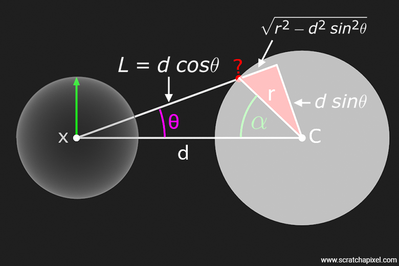
Using \(\alpha\), we can easily calculate where the sample direction intersects the sphere without any fear of failure, using simple geometry. To do so, we will first use the Law of Cosines, which states that for any triangle with sides of lengths \(a\), \(b\), and \(c\), and with \(\alpha\) being the angle opposite the side \(c\), the Law of Cosines states that:
$$c^2 = a^2 + b^2 - 2ab \cos(\alpha)$$You can see from the figure that \(a\), \(b\), and \(c\) are represented by \(d\), \(r\) (the radius of the sphere), and \(L\) (the distance between the shaded point \(x\) and the point on the sphere we are looking at), respectively.
$$L^2 = d^2 + r^2 - 2dr \cos(\alpha)$$It happens that \(L\) can be calculated from the data we have. It's \(d\), the distance between the shaded point \(x\) and the sphere center, multiplied by the cosine of the angle made by the sample direction with respect to the line connecting these two points, minus the opposite side of the smaller triangle depicted in red in the figure. We can also calculate the length of that triangle edge. We know that the hypotenuse of a right triangle is \(c = \sqrt{a^2 + b^2}\). Replacing \(c\) with \(r\) (the sphere radius) and \(a\) with \(d\sin\theta\), we get for that triangle edge:
$$\sqrt{r^2 - d^2 \sin^2 \theta}$$So the length we are looking for is:
$$L = d\cos\theta - \sqrt{r^2 - d^2 \sin^2 \theta}$$From there, we can find that (see the box below for the derivation steps if you want to):
$$\cos(\alpha) = \frac{d}{r} \sin^2 \theta + \cos \theta \sqrt{1 - \frac{d^2}{r^2} \sin^2 \theta}$$The author points out that \( \sin(\theta_{\text{max}}) = \frac{r}{d} \) and so we can rewrite the above equation as:
$$\cos(\alpha) = \frac{\sin^2 \theta}{\sin(\theta_{\text{max}})} + \cos \theta \sqrt{1 - \frac{\sin^2 \theta}{\sin^2(\theta_{\text{max}})}}$$Here is the step-by-step derivation to get to that result:
Given the figure, we have the relationships:
$$ L = d \cos \theta - \sqrt{r^2 - d^2 \sin^2 \theta} $$and by the Law of Cosines,
$$ L^2 = d^2 + r^2 - 2dr \cos(\alpha) $$1. Square Both Sides of the First Equation:
First, let's square the equation for \(L\):
$$ L^2 = \left( d \cos \theta - \sqrt{r^2 - d^2 \sin^2 \theta} \right)^2 $$This gives:
$$ \begin{array}{rl} L^2 & = (d \cos \theta)^2 + \left( \sqrt{r^2 - d^2 \sin^2 \theta} \right)^2 - 2 d \cos \theta \cdot \sqrt{r^2 - d^2 \sin^2 \theta} \\ L^2 & = d^2 \cos^2 \theta + (r^2 - d^2 \sin^2 \theta) - 2 d \cos \theta \cdot \sqrt{r^2 - d^2 \sin^2 \theta} \\ L^2 & = d^2 \cos^2 \theta + r^2 - d^2 \sin^2 \theta - 2 d \cos \theta \cdot \sqrt{r^2 - d^2 \sin^2 \theta} \end{array} $$2. Equate Both Expressions for \(L^2\):
Now, equate this expression to the one derived from the Law of Cosines:
$$ d^2 \cos^2 \theta + r^2 - d^2 \sin^2 \theta - 2 d \cos \theta \cdot \sqrt{r^2 - d^2 \sin^2 \theta} = d^2 + r^2 - 2dr \cos(\alpha) $$3. Simplify the Equation:
First, let's cancel \(r^2\) from both sides:
$$ d^2 \cos^2 \theta - d^2 \sin^2 \theta - 2 d \cos \theta \cdot \sqrt{r^2 - d^2 \sin^2 \theta} = d^2 - 2dr \cos(\alpha) $$Rearrange the terms involving \(d^2\):
$$ d^2 (\cos^2 \theta - \sin^2 \theta) - 2 d \cos \theta \cdot \sqrt{r^2 - d^2 \sin^2 \theta} = d^2 - 2dr \cos(\alpha) $$Recall that:
$$ \cos^2 \theta - \sin^2 \theta = 1 - 2\sin^2 \theta $$This is one of many possible trigonometric identities. So the equation becomes:
$$ d^2 (1 - 2 \sin^2 \theta) - 2d \cos \theta \cdot \sqrt{r^2 - d^2 \sin^2 \theta} = d^2 - 2dr \cos(\alpha) $$Simplify further:
$$ d^2 - 2d^2 \sin^2 \theta - 2d \cos \theta \cdot \sqrt{r^2 - d^2 \sin^2 \theta} = d^2 - 2dr \cos(\alpha) $$Subtract \(d^2\) from both sides:
$$ -2d^2 \sin^2 \theta - 2d \cos \theta \cdot \sqrt{r^2 - d^2 \sin^2 \theta} = -2dr \cos(\alpha) $$Divide by \(-2d\):
$$ d \sin^2 \theta + \cos \theta \cdot \sqrt{r^2 - d^2 \sin^2 \theta} = r \cos(\alpha) $$Divide both sides by \(r\):
$$ \cos(\alpha) = \frac{d \sin^2 \theta}{r} + \frac{\cos \theta \cdot \sqrt{r^2 - d^2 \sin^2 \theta}}{r} $$Finally, express in terms of the ratio:
$$ \cos(\alpha) = \frac{d \sin^2 \theta}{r} + \cos \theta \cdot \sqrt{1 - \frac{d^2 \sin^2 \theta}{r^2}} $$Here is a "raw" implementation of Fred Akalin's method:
Vec3f SphereLight::Sample(const DifferentialGeometry& dg, Sample3f& wi, float &tmax, const Vec2f& sample) const override {
	Vec3f dz = center_ - dg.P;
	float dz_len_2 = dz.Dot(dz);
	float dz_len = std::sqrtf(dz_len_2);
	dz /= -dz_len;
	Vec3f dx, dy;

	CoordinateSystem(dz, dx, dy);

	float sin_theta_max_2 = radius_ * radius_ / dz_len_2;
	float sin_theta_max = std::sqrt(sin_theta_max_2);
	float cos_theta_max = std::sqrt(std::max(0.f, 1.f - sin_theta_max_2));

	float cos_theta = 1 + (cos_theta_max - 1) * sample.x;
	float sin_theta_2 = 1.f - cos_theta * cos_theta;

	float cos_alpha = sin_theta_2 / sin_theta_max + cos_theta * std::sqrt(1 - sin_theta_2 / (sin_theta_max * sin_theta_max));
	float sin_alpha = std::sqrt(1 - cos_alpha * cos_alpha);
	float phi = 2 * M_PI * sample.y;

	Vec3f n = std::cos(phi) * sin_alpha * dx + std::sin(phi) * sin_alpha * dy + cos_alpha * dz;
	Vec3f p = center_ + n * radius_;

	Vec3f d = p - dg.P;
	tmax = d.Length();
	...
}
By "raw" I mean that the code here relies on many divisions and other uses of the cosine and sine functions, which in some situations are numerically unstable. So while this code works for our rather basic scene, it might fall short for scenes presenting corner cases, such as when the sphere light is very small, very far, etc. If you were to use this code in production you'd need to add these checks.
The way we calculate the various variables is rather straightforward since we gave the equations for all of them. The only potentially tricky part is the calculation of the point on the sphere using the \(\alpha\) and \(\phi\) angles. However, by looking at the figure above, you should be able to make sense of it. Note that the point is on the unit sphere centered at the origin (since we only use angles and trigonometric functions to calculate the position), so we need to finally move that point to its final location on the sphere in world space.
That's it. All we need to do to conclude this part of the lesson is replace, at the end of the Sample method, the PDF used for the area sampling method with the PDF for the cone sampling method:
Vec3f SphereLight::Sample(const DifferentialGeometry& dg, Sample3f& wi, float &tmax, const Vec2f& sample) const override {
	...
	float pdf = 1.f / (2.f * M_PI * (1.f - cos_theta_max));
	wi = Sample3f(d / tmax, pdf);
	return Le_;
}
The following image shows a comparison between area and cone sampling with the same number of samples used (64). As you can see, the improvement is rather spectacular. This demonstrates the superiority of the cone sampling strategy when it comes to spherical light.
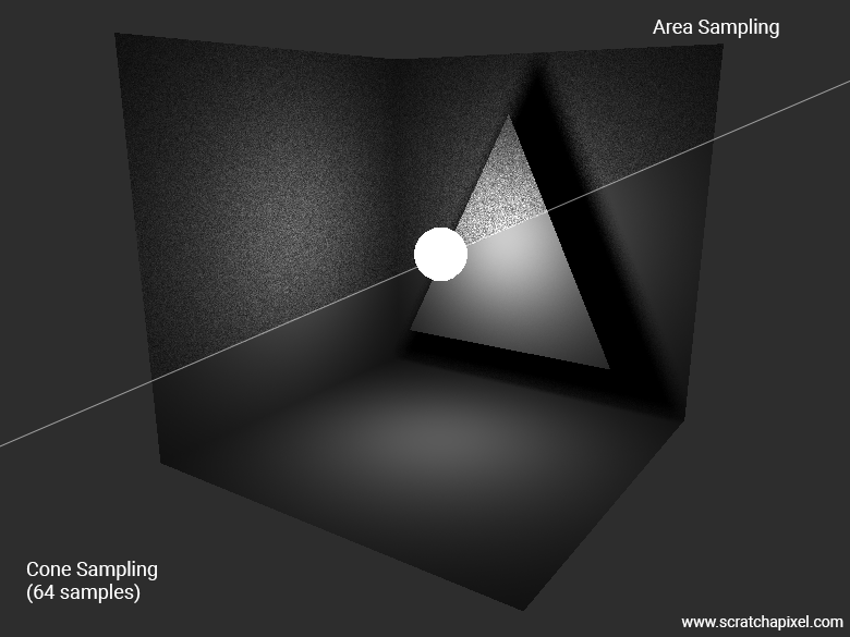
You can alternate between the three methods, of course: area-sampling, cone sampling using the ray-sphere intersection test, and cone sampling using Akalin's method. You should get consistent results in every case (minus the noise, which will be much more noticeable, of course, in the image using the area-sampling method, assuming a constant number of samples).
This lesson has inspired one of Scratchapixel's readers and supporters, Paviel Kraskoŭski, to write a small real-time program that helps visualize the generation of samples using the cone sampling method. Courtesy of Paviel, we show here a video screen recording of his app in action.
Going Further: Get Ready For Part 2
There's much more to cone sampling than what we have covered in this chapter. For example, as mentioned in previous chapters, cone sampling can also be utilized for triangles and quad lights. While we won't demonstrate the implementation of this technique in this particular lesson—considering it already a thorough introduction to the topic—we plan to either introduce a separate lesson or add a new chapter in the future to study this method specifically (we have more urgent topics to cover before doing so). However, let's quickly delve into why cone sampling might be a superior method for triangular and quad lights, especially when they are large relative to the shaded point—meaning they cover a significant portion of the hemisphere above \( x \). At least provide you with an intuition as to why it is the case.
While area sampling is straightforward for shapes like triangles and quads, the following figure illustrates why it may not be optimal. The figure shows a large rectangular area light parallel to a shaded surface (front orthographic view). It's evident that as we take several uniformly distributed samples over the surface of this area light, their contribution is attenuated by the two Lambert cosine terms used in the equation: the cosine of the angle between the light sample direction and the light surface normal, and the cosine of the angle between the sample direction and the shaded point surface normal. Additionally, points further away from the shaded point contribute less due to the square distance falloff. The figure demonstrates that when samples are uniformly distributed across the light's surface and projected onto the hemisphere above \( x \), those contributing less are more densely packed than those contributing more. As the area light extends further on both sides of the hemisphere, the density increases, particularly towards the horizon. This distribution is clearly suboptimal.
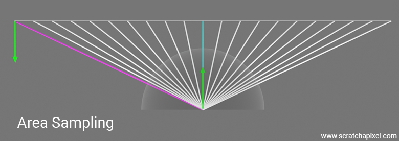
Technically, or ideally, we should aim for a distribution of samples that has a probability \( p(x') \) according to \( (\omega \cdot n')||x-c||^{-2} \) or, even better, \( (\omega \cdot n)(\omega \cdot n')||x-c||^{-2} \), where \(\omega\) is the sample direction, \(x'\) the sample on the area light, and \( n \) and \( n' \) are the surface and light normals, respectively. As you can see, this probability distribution function would consider both distance and the two cosine terms involved in the rendering equation.
One (easy) approach to mitigate this issue with area sampling is to uniformly sample the solid angle subtended by the light instead, which should intuitively provide better results. With this method, there are fewer samples contributing less to the shaded point illumination compared to the area sampling method. This indicates why sampling the cone angle, even for rectangular and quad lights, is better, especially when the lights are large relative to the hemisphere above the shaded point \(x\).

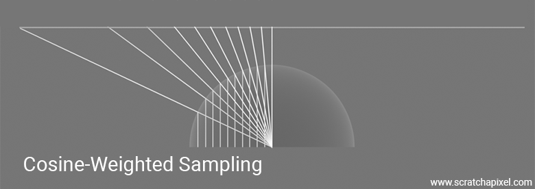
An even more effective but harder distribution method involves uniformly sampling the projected solid angle itself. This method is beneficial because it produces samples that, once projected onto the solid angle, are distributed in proportion to their contribution with respect to the cosine term—a cosine-weighted distribution. Despite its effectiveness, this method is not as commonly used due to its implementation complexity. Therefore, many opt for the simpler solid angle sampling method.
These techniques are out of the scope of an introductory lesson on lights and area lights. They are considered advanced methods and can be quite hard to implement (at least for the projected solid angle method) and more computationally expensive. However, considering that there's more to cover on the topic of lights in general, we have already planned a part 2 to this lesson, in which we will study these methods specifically (and more).
In addition, the main issue with using the Monte Carlo method is the resulting noise in the image, which is due to the fact that there's a strong variance between adjacent samples. Variance refers to the difference between the ground truth result and the approximation provided by the Monte Carlo estimation. The more samples there are, the lower the variance, but the higher the computational cost. Therefore, while the Monte Carlo method is quite simple in principle and easy to implement in practice, the bulk of the work, and where it gets slightly harder, is in developing techniques for reducing that noise or variance for a constant number of samples. These techniques cover a wide range of mathematical methods and names but are generally referred to as variance reduction methods, a subset of which being importance sampling. As we progress in our lessons, we will eventually study these topics.
Though be patient, as some lessons from the basic section are yet to be covered before we can get to these advanced topics. We have already covered significant ground in this lesson, including making you aware of these more advanced methods to hopefully keep you busy until then.