Introduction to Lighting

Spherical Area Light: Using Area Sampling

Preamble

Because each shape that an area light can have has its own specific implementation considerations, we have decided to dedicate one page per area light shape. More specifically, we will consider triangular, planar, disk, and finally spherical area lights. This preamble is repeated on each page to ensure that if you landed on one of these pages from an external link, you are aware that it is advisable to start by reading the page on the triangular area light. There, we will discuss some concepts that will be reused across the other light types and provide a general explanation about the code we will be using to implement these lights.

Also note that we strongly recommend that you read the lessons on Distributed Ray-Tracing and Stochastic Sampling and Sampling Strategies, which are corollaries to this one.

What Will You Learn in this Chapter?

As mentioned in the chapter on triangular area lights, unlike the chapter on quad lights which wasn't very different from triangular lights, implementing spherical area lights will give us an opportunity to delve into a different method of evaluating the contribution of area lights called cone sampling. Therefore, we strongly encourage you to read this chapter as carefully as you did the lesson on triangular area lights, as key concepts will be introduced here.

This chapter is divided into two main parts:

• Implementing Spherical Area Lights Using Area Sampling: In the first part, we will learn how to implement spherical area lights using the area sampling method, which we have studied in the last two chapters. Although we will learn new critical aspects of the ray-tracing method in this section, read it carefully even if you feel familiar with the concepts from the previous chapters.

• Learning About Cone Sampling: The second part is devoted to learning about cone sampling, another method that can be used to sample area lights.

Uniform Sampling of a Spherical Light

Similarly to how we've implemented the triangular area light, implementing spherical area lights using the area sampling method requires finding a way to sample spheres.

For the purposes of debugging, a constant density function is useful. (Peter Shirley, Changyaw Wang - Monte Carlo Techniques for Direct Lighting Calculations).

The quote above is from Peter Shirley and Changyaw Wang in their paper entitled "Monte Carlo Techniques for Direct Lighting Calculations" (see the references section at the bottom of the page). This simply means that the most basic way of sampling a spherical light is by using a uniform distribution, similar to how we sampled quad and triangular lights. This involves starting with a sample uniformly distributed on the unit square, mapping it to the sphere, and using a probability density function (PDF), which in this case is \( \frac{1}{\text{area}} \). As we know, the area of a sphere is \( 4\pi r^2 \). So far, this seems rather simple.

As with the naive method that we started with for uniformly sampling a triangle, we can ask ourselves: how would you map that sample on the unit square to the sphere?

The first thing we need to do is define a Cartesian coordinate system and a convention to define the position of a point on the sphere using spherical coordinates. When it comes to both Cartesian and spherical coordinate systems, you might come across different conventions. Here is the definition of the conventions we will be using in this chapter:

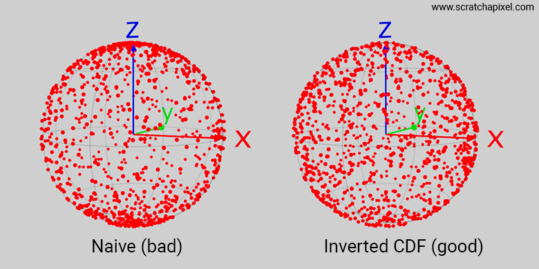
• Cartesian Coordinate System: While this is not our preferred convention, we decided to use it. Most papers written in the 90s (or earlier) related to sampling shapes such as spheres use these conventions, and because of that historical background, many people, particularly those with a background in mathematics, keep using it today. So while this is not our preferred convention, to stay consistent with the papers we will reference at the bottom of the page, we will stick to this. In this convention, \(z\) is up, the \(x\)-axis of the Cartesian coordinate system points to the left, and the \(y\)-axis points away from you (or from the screen, as shown in Figure 1).

• Spherical Coordinates: The papers we've been alluding to also use a convention that is the opposite of what we tend to use on the website (and more generally in more recent research papers and books devoted to computer graphics). While we do not particularly encourage you to use this convention, we will stick with it for now because you might read papers using it in the future, and it's good to be aware that different authors might use different conventions. So for the sake of this lesson, the angle \(\theta\) (Greek letter theta) will refer to the azimuthal (longitude) angle and will vary from 0 to \(2\pi\). The angle \(\phi\) (Greek letter phi) will be the polar or elevation (latitude) angle and will vary from 0 to \(\pi\). Note that the positive \(z\)-axis is \(\phi = 0\) and the positive \(x\)-axis is \(\theta = 0\).

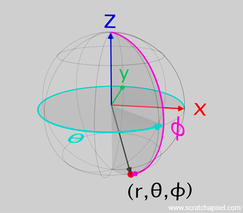
With these conventions set, here are the equations that we will be using to convert a point in spherical coordinates to Cartesian coordinates (again, refer to Figure 1). For clarity, we've added the subscript \(az\) for azimuthal and \(el\) for elevation (also known as the polar angle of latitude):

Vec3 SampleUnitSphereNaive(float r1, float r2) {
	float theta = 2 * M_PI * r1; // azimuthal angle
	float phi = M_PI * r2; // polar angle
	return { 
		std::cos(theta) * std::sin(phi), 
		std::sin(theta) * std::sin(phi),
		std::cos(phi) };
}

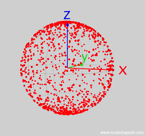
The result visible in Figure 2 clearly shows that with this approach, there is a concentration of samples near the poles. We will explain shortly why this is happening, but in a broader scope, the reason is similar to the problem of remapping samples on the unit square to the triangle. We spoke about the Jacobian being the scale factor applied when you transform one "shape" (the unit square) to another (the triangle). For the uniform distribution property to remain uniform after transformation, the Jacobian needs to be constant. The issue with the way we are remapping the samples from the unit square to the sphere using this basic approach is precisely that the Jacobian is not constant. One way to understand this is to consider a small differential area on the sphere parameterized in terms of spherical coordinates. Let's look at the equation and break it down:

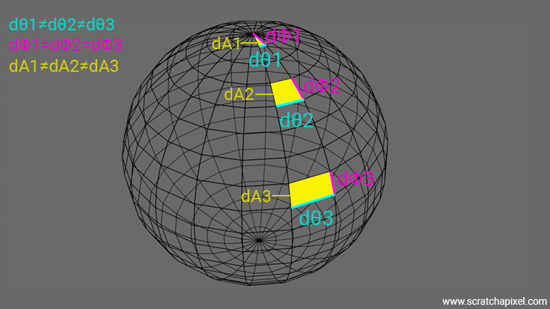
where \(r\) in the above equation stands for the sphere's radius. The idea is to take a small differential angle in both \(\theta\) and \(\phi\), which, when multiplied by each other, would give you the area of a small patch on the surface of the sphere. You can see a representation of this small differential area and the terms used to calculate it in the following figure:

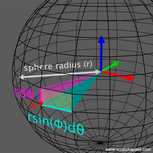
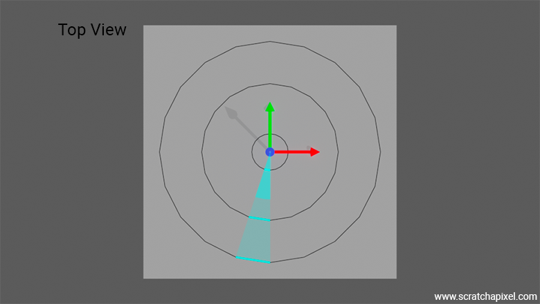
Basically, if you imagine that we want to determine a small differential area at point \(x\) on the sphere as shown in the figure. It doesn't matter if \(x\) is centered with respect to that small differential area (the transparent yellow patch in Figure 3) or to the side of it as represented in Figure 3. The concept is the same regardless. Now, the position of \(x\) on the sphere in terms of spherical coordinates is \(\theta\) (azimuthal) and \(\phi\) (polar). The sphere has a radius \(r\). So from \(x\), we move up by a tiny fraction \(\phi\), hence the \(d\phi\) multiplied by the sphere radius. In the end, this gives us \(\textcolor{magenta}{r d\phi}\). And we do the same thing with \(\theta\), so technically we could write \(r d\theta\). However, note that for any given \(d\theta\), the length of the given horizontal segment (the segment highlighted with the cyan color in the figure) varies with \(\phi\). The closer we are to the pole, the smaller the segment; the closer we are to the equator, the larger the segment. This can be seen in the following figure, which gives a view of the sphere rendered from the top, where from the sphere, we've only represented three of such possible longitudinal lines. Within a given small differential angle for \(\theta\), we can see that the segment along the sphere equator is larger than those that are close to the pole.

The length of these segments is proportional to the radius of the sphere where these segments are being created, and this radius is given by \(r \sin(\phi)\). This can be more easily understood if you look at the following figure, in which we show that the inner circle (in grey) has a radius \(r \sin(\phi)\), from which we can see that the segment length is \(\textcolor{cyan}{r \sin(\phi) d\theta}\).

The area of the small differential area being the product of these two segments (the one we got by moving along \(\phi\) and the one we got by moving along \(\theta\)) is indeed \(dA = \textcolor{cyan}{r \sin(\phi) d\theta} \, \textcolor{magenta}{r d\phi} = r^2 \textcolor{cyan}{\sin(\phi) d\theta}\textcolor{magenta}{d\phi}\).

As a consequence of this, you can easily see by looking at the following figure that differential areas near the pole are much smaller than those near the sphere's equator. This explains why our remapping process doesn't work. The process we've been using to transform the unit square to a sphere doesn't preserve area (the Jacobian is not constant). Therefore, as the area gets squeezed towards the poles, we get a concentration of samples in these regions.

We've learned why this doesn't work, but then can we make it work? Hopefully yes. To understand how to solve this problem, we need to delve into the theory of probabiliy which is what we are going to do next. Take your time to read the following content, as it will set some key techniques that you will come across over and over in 3D rendering.

Sampling a Non-Uniform Probabiliy Density Function: A Dive in Probability Theory

Objective: Our objective is to use two uniformly distributed random numbers, \(\varepsilon_1\) and \(\varepsilon_2\), to generate samples uniformly distributed across the surface of a sphere. The positions of these samples will be defined by their spherical coordinates \(\theta\) and \(\phi\).

The problem we face is that, intuitively, without even knowing the specifics of the function, one can easily understand that the result of sampling the sphere using a uniformly distributed pair of random numbers leads to a non-uniform distribution of samples (due to the density function \(dA\)). We have a higher concentration of samples at the poles.

Our goal is to cancel out this higher concentration of samples at the poles so that the final distribution of samples over the sphere is uniform. For that, we will need to resort to a method that was initially developed and used in the 1950s. Remember that the probability of a uniform sampling distribution of samples across the surface of the sphere is:

where \(x\) marks the sample, and \(p(x)\) indicates the probability of that sample being chosen (which, in this case, as we know, is uniform). The density function of the sphere parameterized in terms of \(\theta\) and \(\phi\) is:

The first equation ensures equal probability per unit area over the sphere's surface. The second equation indicates how the area changes with \(\theta\) and \(\phi\). Hold on to these two descriptions. Now if we combine the two together, that is, we write:

This function is a valid probability density function in the sense that it can be integrated over the sphere to give 1, representing the total probability, i.e., certainty that a point lies on the sphere's surface. We showed in the note above that integrating the differential area over the range \(0 \leq \theta \leq 2\pi\) and \(0 \leq \phi \leq \pi\) results in \(4\pi r^2\). That combined density describes how the probability is distributed over the surface of the sphere in terms of the spherical coordinates \(\theta\) and \(\phi\).

Now we can look at this equation \(p(\theta, \phi)\) as being essentially made of two parts:

• \(p(\theta) = d\theta\)

• \(p(\phi) = \sin(\phi)d\phi\)

These densities are expressed with their differential elements. The term \(d\theta\) suggests that \(\theta\) is uniformly distributed over its domain \([0, 2\pi]\). The term \(\sin(\phi) d\phi\) suggests a non-uniform distribution over \([0, \pi]\). We need to integrate them over their respective domains \([0, 2\pi]\) and \([0, \pi]\) to handle normalization. Normalization ensures that the total probability over the entire space sums to 1. Without normalization, the probability densities might not integrate to 1, leading to an incorrect representation of the distribution (this will make more sense very soon).

Let's first integrate \(p(\theta)\):

Therefore, \(p(\theta) = \dfrac{1}{2\pi}\). Now let's go through the same process for \(\phi\). Let's integrate its differential form:

Therefore, \(p(\phi) = \dfrac{\sin(\phi)}{2} \).

It's really important to understand this part. If we haven't explained it clearly enough, please let us know, and we will try to rephrase it until you understand.

The reason why we've separated these two functions in the first place is because, in this particular case:

So, the probability of drawing a sample with spherical coordinates \(\theta\) and \(\phi\) (where both of these numbers are random variables) is equal to the product of the probability of drawing \(\theta\) and the probability of drawing \(\phi\). In mathematics (and probability theory), this is called a joint probability and \(p(\theta)\) and \(p(\phi)\) are called marginal probabilities (or distributions). We said "in this particular case" because \(\theta\) and \(\phi\) are independent variables (in this particular case). This technique couldn't be used if these random variables were not independent.

Remember what our objective is: we can generate random numbers uniformly sampled in the range [0,1], and we want to use them to come up with values for \(\theta\) and \(\phi\) in such a way that the resulting samples will be uniformly distributed across the surface of a sphere. Remember also that the PDF provides the likelihood of a random variable taking the value \(x\). The PDF describes a density of probability or how densely the probability mass is distributed at each point in the domain.

There's another useful function in probability theory called the cumulative density function or CDF, which can be built from the PDF. We will explain how in a moment, but for now, we will first understand what the CDF is. Assuming you have a CDF, \(F(x)\), defined as:

This function gives the probability that a random variable \(X\) is less than or equal to \(x\). To be clear, you somehow draw a random number, say 5, and you want to know the probability that any of the possible dice outcomes will be lower or equal to 5. The \(X\) are the numbers on the dice (all the possible outcomes), which is a random variable since each time you throw the dice, you get a different number. You draw another random number, 5, that's your \(x\), and you want to know the probability that you get a number lower or equal to 5 when you throw the dice on the table. If you are comfortable with that example, which is rather simple, you might have already guessed that this probability is the sum of the probabilities of getting a 1, a 2, a 3, a 4, or a 5. That is 5 times \(1/6\), which is \(5/6\). This example uses discrete random variables, but for continuous ones, we can formalize this by writing that the CDF of a probability density function (PDF) is the integral of the PDF. Just as a sum is used for discrete random variables, an integral is used for continuous variables. The CDF represents the probability that the random variable \(X\) takes on a value less than or equal to a specific value \(x\).

Mathematically, the CDF \(F(x)\) is defined as:

In this integral, \(t\) is the variable of integration, and \(x\) is the upper limit of integration, representing the value up to which we calculate the cumulative probability.

For a continuous random variable, the CDF is the integral of the PDF from the lower bound of the random variable's range (negative infinity in the example above) to the value of interest \(x\). This process accumulates the probabilities up to that point. While this can be a bit abstract at first, let's give an example. Imagine we have the following PDF: \(\lambda e^{-\lambda x}\). This PDF integrates to 1, and the proof of that is given in the box below if you are interested, so it can effectively be considered a valid PDF.

To keep things simple, we will write a simple program that helps plot both the PDF and the CDF for the range [0,5]. To do so, we will evaluate the PDF for small steps of \(x\) going from 0 to 5, and for each step, set the CDF as the sum of all the PDFs we have calculated at the preceding steps, plus the current PDF value multiplied by the step size (the \(dt\) in the equation \(\int_{-\infty}^{x} p(t)dt\), see below).

#include <stdio.h>
#include <math.h>

double pdf(double x, double lambda) {
    return lambda * exp(-lambda * x);
}

int main() {
    double lambda = 1.0;  // Rate parameter
    double step = 0.1;    // Step size
    double x, pdf_value, cdf_value = 0.0;

    printf("x\tPDF\t\tCDF\n");

    for (x = 0.0; x <= 5.0; x += step) {
        pdf_value = pdf(x, lambda);
        cdf_value += pdf_value * step;  // Accumulate the CDF

        printf("%0.6f\t%0.6f\t%0.6f\n", x, pdf_value, fmin(cdf_value, 1.0));
    }

    return 0;
}

The following image shows a plot of these two graphs: the PDF of \(p(x) = \lambda e^{-\lambda x}\) on the left, and its resulting CDF on the right.

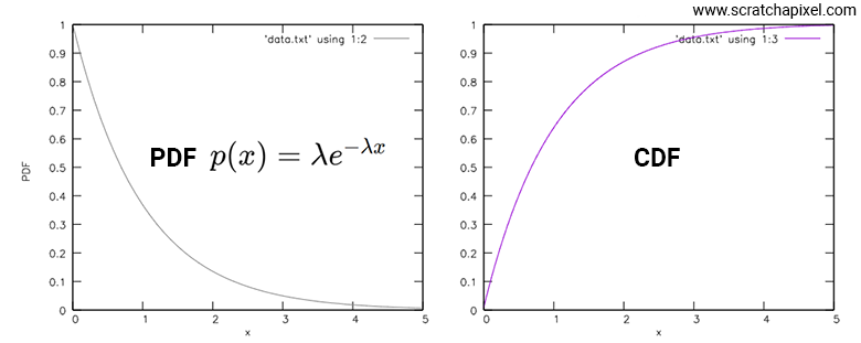
You might be surprised that the CDF doesn't start with the same value as the PDF at \(x\) because we suggested the CDF was equal to whatever its counterpart PDF at \(x\) was plus the sum of all preceding probabilities (preceding \(x\)). That works for discrete random variables, but for continuous random variables, in the integration process, you need to account for the \(dt\) term, which if you use the Riemann sum numerical method for evaluating that integral, as we did in our program, would be represented by the code's step variable. So each time you add the current CDF for the current \(x\), you need to multiply that value by step, which is why the CDF starts much lower.

That being said, what's more interesting about the CDF curve are the following points:

• It never goes above one: Of course, since the CDF represents the probability of a number being lower than any of the outcomes a random variable \( X \) can take, the maximum value a CDF can take is necessarily in the range [0,1].

• The curve is not linear: Naturally, it's not linear because the PDF is not linear either. Therefore, it reflects the non-linearity of the function it was derived from. More on that in a moment.

• The curve is monotonically increasing (or non-decreasing, as some prefer to say): This property is key for various reasons, which we will discuss shortly.

With this being said, and before we explain how to exploit the above properties, let's see how this applies to our sphere-uniform-sampling problem. The equation we want the CDF of is \( p(\phi) = {\sin(\phi)}/{2} \). Let's apply the recipe to get the CDF, which involves integrating this function from the lower bound of \(\phi\) (which is 0) to some value \(\phi\).

• The given PDF is \( p(\phi) = \dfrac{\sin(\phi)}{2} \).

• The CDF, \( F(\phi) \), is defined as the integral of the PDF from the lower bound of \(\phi\) (which is 0) to some value \(\phi\): \( F(\phi) = \int_{0}^{\phi} \dfrac{\sin(\phi')}{2} \, d\phi' \).

• To find the CDF, we need to integrate the PDF: \( F(\phi) = \int_{0}^{\phi} \dfrac{\sin(\phi')}{2} \, d\phi' \).

• We can perform the integration step-by-step:

  $$F(\phi) = \frac{1}{2} \int_{0}^{\phi} \sin(\phi') \, d\phi'$$ $$F(\phi) = \frac{1}{2} \left[ -\cos(\phi') \right]_{0}^{\phi}$$

• Evaluate the definite integral by substituting the limits:

  $$F(\phi) = \frac{1}{2} \left( -\cos(\phi) - (-\cos(0)) \right)$$

  Since \(\cos(0) = 1\), this simplifies to:

  $$F(\phi) = \frac{1}{2} \left( -\cos(\phi) + 1 \right)$$

  Simplifying further, we get:

  $$F(\phi) = \frac{1}{2} \left( 1 - \cos(\phi) \right)$$

The CDF for the given PDF is:

Let's plot this equation over the domain covered by \(\phi\) (0 to \(\pi\)).

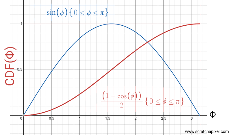
The curve we are interested in is the one in a reddish color. We've added the plot of the sine function within the same range (0 to \(\pi\)) so you can compare the two and see how the CDF relates to the original PDF. Not surprisingly, this red curve has a slower slope at the beginning and end, which is where \(\phi\) approaches the poles. A shallower slope indicates that the probability of our random variable \(X\) being in these ranges is lower than in areas where the curve is steeper. In conclusion, this CDF shows that the probability of having a random variable \(X\) around the poles is indeed lower than elsewhere on the sphere, which is what we are looking for.

Now, the reason why this CDF is wonderful is that it gives us the probability (the value on the y-axis of the plot) that a random variable \(X\) (assumed to be uniformly distributed over the surface of the sphere) has an angle \(\phi\) lower or equal to a value you pick at random (within the range 0 to \(\pi\)). Pay attention here: the value on the y-axis goes from 0 to 1, and on the x-axis from 0 to \(\pi\). The curve that maps these two conforms to the distribution of uniformly distributed samples on the sphere.

So, what do we know and what are we looking for? We know we can generate a uniformly distributed random number in the range 0 to 1. What we are looking for is a number in the range 0 to \(\pi\) such that when we map the first number to the second number (the angle \(\phi\)), the obtained angle \(\phi\) guarantees a uniform distribution of samples over the sphere. Bingo! What we need is not the CDF \(F(x)\) but its inverse function, \(F^{-1}(x)\), which takes a uniformly distributed random number in the range [0,1] and gives us a value for \(\phi\).

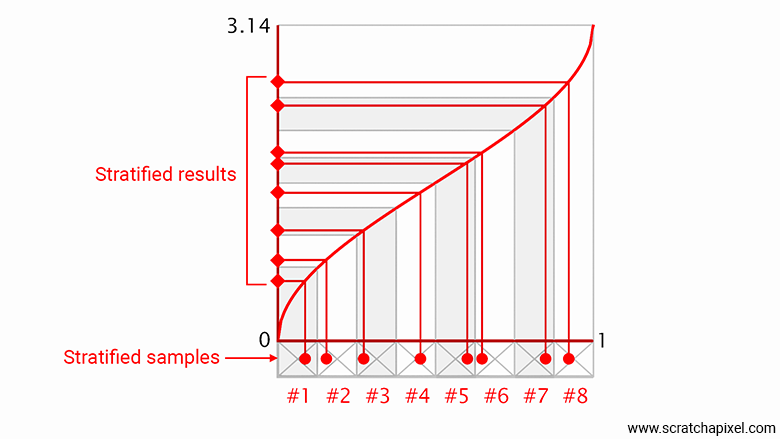
This also works because the CDF has the properties we mentioned above, particularly the monotonic increasing property. This means that when you use the inverse of the function to map a value from 0 to 1 to \(\phi\), the function has one and only one solution. This wouldn't work otherwise. The fact that the function is monotonic increasing also has a very cool benefit that we won't delve into in this lesson because it is explained in detail in the lesson Sampling Strategies. That cool property is that stratified samples remain stratified when we pass them through the \(F^{-1}(x)\) function. Stratified sampling is a noise reduction technique for the Monte Carlo method. In short, the idea consists of dividing your 0-1 range into cells (as many cells as needed samples) and jittering the sample within these cells. By doing so, your samples get stratified as shown in the figure below. Stratified input samples remain stratified when mapped to \(\phi\) using the inverse of the CDF, which is a property we want our remapping method to have. If this wasn't the case, we would lose the benefit of stratified sampling, effectively increasing, rather than reducing, the noise we would get from using Monte Carlo integration. This is why using the inverse of the CDF is such a cool and powerful method.

The following figures, if you are not familiar with the concept of stratified sampling, show an example of what happens when you sample the inverse CDF using stratified samples. The idea behind stratified sampling is to organize the samples into strata, the small cells that we have represented below the x-axis. The cross within each cell indicates the center of the cell. If the samples were perfectly spaced, they would be located at the centers of the cells. This might seem like a good strategy because, by doing so, we would be sure to cover the entire spectrum of the inverted CDF, contrary to using a random sampling strategy which might leave gaps (as a result of being random). However, using regularly spaced samples breaks the theory behind Monte Carlo sampling which expects samples to be randomly uniformly distributed. So, what we do with stratified sampling is a sort of compromise between the two. We create samples within the strata ensuring we cover the entire spectrum of the function sampling space, but we randomly jitter the position of the samples within the strata. This way, we effectively end up with samples that are random but are more likely to be "more regularly" spaced than if we had chosen the purely uniformly random distributed process. While the method explained here is called jittering, more sophisticated processes for placing the samples within the strata exist and will be covered in the lesson on Sampling Strategies.

Now that you at least have a high-level view of what stratified sampling is, it's important to note that when stratified samples are used, the results of using these samples in the inverted CDF are also stratified. As stated above, this is why this method is so effective. We've mentioned it already, but now we have illustrated that concept.

Here are the steps for inverting the CDF in the case of sphere sampling:

That's it! Isn't this really, really cool? So now, all you need are two random numbers in the range [0,1], and you can sample both \(\theta\) and \(\phi\).

All samples generated with this method will be uniformly distributed on the sphere. Let's implement this first by examining a distribution of samples on the sphere, and then by implementing the method for our area light sampling method.

// convention (not recommended):
// - phi: polar angle
// - theta: azimuthal angle
Vec3 SampleUnitSphereGood(float r1, float r2) {
    float phi = std::acos(1 - 2 * r2); // polar angle
    float theta = 2 * M_PI * r1; // azimuthal angle
    return { 
        std::cos(theta) * std::sin(phi), 
        std::sin(theta) * std::sin(phi),
        std::cos(phi) 
    };
}

Note that when it comes to code, you can use 1 - 2 * r2 directly in place of std::cos(phi). This saves a call to std::acos and std::cos. From there, we can also easily precompute \(\sin\phi\) knowing that \(\cos^2\phi + \sin^2\phi = 1\), and so \(\sin\phi = \sqrt{1 - \cos^2\phi}\). Therefore, the code can be made a bit faster with:

// convention (not recommended):
// - phi: polar angle
// - theta: azimuthal angle
Vec3 SampleUnitSphereGoodAndFaster(float r1, float r2) {
    float z = 1 - 2 * r2; // this is cos(phi)
    float sin_phi = std::sqrt(1 - z * z); // this is sin(phi) = sqrt(1 - cos^2(phi))
    float theta = 2 * M_PI * r1; // azimuthal angle
    return { 
        std::cos(theta) * sin_phi, 
        std::sin(theta) * sin_phi,
        z 
    };
}

// convention (recommended):
// - theta: polar angle
// - phi: azimuthal angle
inline Vec3f UniformSampleSphere(const float& r1, const float& r2) {
	float z = 1.f - 2.f * r1; // cos(theta)
	float sin_theta = std::sqrt(1 - z * z);
	float phi = 2 * M_PI * r2; // azimuthal angle
	return {std::cos(phi) * sin_theta, std::sin(phi) * sin_theta, z};
}

SphereLight Implementation

In order to proceed, we need to add a Sphere class to our code. We invite you to look at the code to see the details of this class implementation. As there's nothing special to it, we will save some space here. But in a few words, this class is derived from the class TriangleMesh. When an instance of the sphere is created, the Sphere's class constructor calls a private Triangulate method which in turn fills the TriangleMesh member variables with the proper data to represent this sphere as a triangle mesh. In a production renderer, you'd probably want to implement some screen-based tessellation method, so that the object appears as a perfectly smooth sphere (as opposed to faceted). There are a couple of methods for doing so: one can be inspired by the REYES algorithm, the other would consist of representing the sphere as an icosahedron which we would subdivide until every triangle making the sphere would approximately be 1 pixel in screen space. As mentioned, we won't be looking into these methods (at least for now). We might come back to this part of the lesson in a future revision.

The SphereLight class implementation looks like so:

class SphereLight : public AreaLight {
public:
	SphereLight(Vec3f center = 0, float radius = 1, const Vec3f& Le = 1)
		: AreaLight(Le)
		, center_(center)
		, radius_(radius)
		, sphere_(new Sphere(center, radius)) {
	}

	std::shared_ptr<Light> Transform(const Matrix44f& xfm) const override {
		Vec3f xfm_center;
		Vec3f scale;
		ExtractScaling(xfm, scale);
		assert(scale.x == scale.y && scale.x == scale.z);
		xfm.MultVecMatrix(center_, xfm_center);
		return std::make_shared<SphereLight>(xfm_center, radius_ * scale.x, Le_);
	}

	std::shared_ptr<Shape> GetShape() override { return sphere_; }

	Vec3f Sample(const DifferentialGeometry& dg, Sample3f& wi, float &tmax, const Vec2f& sample) const override {
		Vec3f n = UniformSampleSphere(sample.x, sample.y);
		Vec3f p = center_ + n * radius_;
		Vec3f d = p - dg.P;
		tmax = d.Length();

		float d_dot_n = d.Dot(n);
		if (d_dot_n >= 0) return 0;

		wi = Sample3f(d / tmax, (2.f * tmax * tmax * tmax) / std::abs(d_dot_n));

		return Le_;
	}

private:
	Vec3f center_{0};
	float radius_{1};
	std::shared_ptr<Sphere> sphere_;
};

The methods are the same as those we already presented for our TriangleLight.

• When an instance of the Sphere is created, the class constructor creates an instance of the sphere as a triangular mesh. This is also where we set the default sphere radius and center for the light itself (which are, of course, similar to those of the light as a mesh). By default, the sphere is created at the world's origin with a radius equal to 1. It is only when the Transform method is called during scene construction that we effectively generate an instance of the same light but in its final position and with its final radius, which can be affected by the matrix scale value.

  Going through a two-step process is a design choice that allows us to support a form of instancing in which a shape that you might want to duplicate multiple times in the scene is first generated with its "default" settings (such as, for example, in this case, a sphere with radius 1 centered at the world origin). Then, each instance of that object is obtained in a second phase by generating a mesh that is the result of the original mesh transformed by a given matrix.

  The rationale behind this design is explained in the lesson Core Components to Build a Ray-Tracing Engine from Scratch: A DIY Guide.

  Note that while we agree that the matrix can scale the light up or down, we only agree for a matrix that does so uniformly across all axes (aka uniform scaling). The solution to extract the scale value from the rotation value (which shall not affect our sphere area light) is to call the ExtractScaling matrix helper method. Remember that a transformation matrix can be seen as a Cartesian coordinate system that is a system whose axes are orthogonal to each other. In a row-major matrix (which is the convention we use on Scratchapixel), each of the first three rows represents the x-, y-, and z-axis of this Cartesian coordinate system. So, all the ExtractScaling method needs to do to extract the x, y, and z scaling values encoded by the transformation matrix is to calculate the length of these axes. Simple.

  template<class T>
  void ExtractScaling(const Matrix44<T>& mat, Vec3<T>& scale) {
      Vec3<T> row[3];
  
      row[0] = Vec3<T>(mat[0][0], mat[0][1], mat[0][2]);
      row[1] = Vec3<T>(mat[1][0], mat[1][1], mat[1][2]);
      row[2] = Vec3<T>(mat[2][0], mat[2][1], mat[2][2]);
  
      scale.x = row[0].Length();
      scale.y = row[1].Length();
      scale.z = row[2].Length();
  }
  

• The Sample method is where we remap two random values uniformly distributed in the range [0,1] to spherical coordinates. UniformSampleSphere generates a sample on the unit sphere, so we need to transform it into its final world position, which we can simply do by multiplying the sample by the sphere radius and adding the sphere center position. Since we ignore the sphere rotation (see below), we can then use the sample position on the unit sphere as our normal (which has unit length).

  In the implementation we provide in this lesson, we've indeed ignored rotation. If your sphere remains of uniform color, that's not so important because a sphere looks like a sphere regardless of its rotation. However, if you were to texture the Le_ parameter of the light, then we would obviously need to take rotation into consideration. But the crux of the matter for this lesson is really more about learning how to sample area lights of various shapes rather than making a production renderer. So, if you are interested in adding rotations, it will be something that you will need to implement yourself, but it shall be super simple: you just need to store the transformation matrix applied to the light during instantiation (when the Transform is being called) as a member variable of the class alongside the matrix inverse. Then, when a sample is generated, you can simply apply the transform matrix to transform the sample position to its world position (which will include rotations potentially encoded by the matrix). To calculate the normal, you will need to transform the sample position by the matrix inverse. And with that, you shall get rotation support. Again, Scratchapixel's philosophy is to keep the sample code that comes with each lesson as small as possible, no need here to go through these details which do not directly relate to area light implementation.

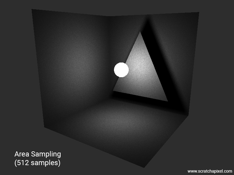
Here is the output of our sample program using the area sampling method for the sphere light with 512 samples:

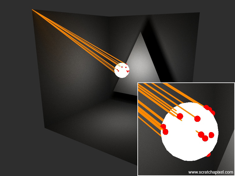
Why Isn't Area Sampling Ideal for Sphere-Shaped Area Lights?

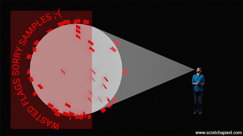
The problem with this method is that some of the samples generated are not being used, since-at least- half of the samples are not directly visible from the shaded point's point of view. It's like planting a flag on the moon and counting how many flags you can see from the Earth. The team with the most flags visible from the earth wins. Well, if you put flags on the far side of the moon or beyond the viewer's line of sight, that’s not a very effective strategy. Hopefully, you'll agree that we are wasting a lot of samples here! That’s why this method is not great.

Say Hello to Cone/Angle Sampling!

The problem with this method is that some of the samples generated are not being used, since at least half of the samples are not directly visible from the shaded point's point of view. It's like planting flags on the moon and counting how many flags you can see from Earth. The team with the most flags visible from Earth wins. Well, if you put flags on the far side of the moon or beyond the viewer's line of sight, that’s not a very effective strategy. Hopefully, you'll agree that we are wasting a lot of samples here! That’s why this method is not great.

Hopefully, there is a better way of sampling the sphere that doesn't suffer from this issue. This method involves sampling directions within the cone of directions subtended by the sphere as seen from the shaded point. This technique, referred to as cone and solid angle sampling, will be detailed in the next chapter.

References

Peter Shirley, Changyaw Wang - Monte Carlo Techniques for Direct Lighting Calculations.